Simio and Simulation: Modeling, Analysis, Applications - 7th Edition
Chapter 13 AI-enabled Simulation Modeling
Note: This chapter was originally written and contributed by Mohammad Dehghani and Rylan Carney
The concept of Digital Twin (DT) plays a crucial role as a significant enabler for Industry 4.0 initiatives. In this transformative era, organizations increasingly recognize the pivotal role of Digital Twin in optimizing operations and facilitating data-driven decisions. This virtual replication of physical assets and systems empowers businesses to achieve greater efficiency and flexibility.
With technological advancements driving the enhancement of digital twin tools, the integration of Artificial Intelligence (AI) emerges as a transformative force in this rapidly evolving landscape. AI elevates the intelligence and adaptability of digital twins, making them even more invaluable in Industry 4.0 initiatives. AI, driven by machine learning and predictive analytics, empowers digital twins to adapt to changing conditions as required. They can identify patterns, predict potential issues, and proactively recommend optimal solutions. Leveraging AI allows organizations to maximize the potential of their digital twins, streamlining operations, minimizing downtime, and enhancing overall efficiency.
Simio stands as the pioneer among discrete event simulation software by incorporating built-in support for neural networks, unlocking AI’s power to enhance Digital Twin models. This allows users to employ neural networks for inference within model logic and simplifies the capture of training data and offers an intuitive interface for training neural network models. This offers users to:
Create feedforward neural networks without coding, reducing model development time.
Improve decision-making, optimizing production cycles, resource management, and capacity planning.
Implement predictive analytics to minimize downtime and its associated impacts.
Import trained neural network ONNX files into Simio, enhancing model intelligence.
Simio first introduced embedded neural networks and related tools in Simio version 14.230 (released October 2021) and has continued regular enhancements. This chapter aims to provide a tutorial on using this tool and deploying trained models as decision-making modules in simulations.
13.1 Digital Twin Levels
Since applying AI-enabled techniques such as neural networks within a simulation environment is a newly developed concept, it is important to explore their application within different levels of Digital Twins. This understanding will help grasp the trajectory of Digital Twin evolution and the strategic placement of neural network tools.
A journey toward a digital twin can be undertaken in 5 levels: 1-Supervision, 2-Experimentation, 3-Optimization, 4-Prediction, and 5-Automation (see Figure 13.1). Depending on their needs, different organizations should tailor their Digital Twin level to align with their operational requirements and decision-making processes. It is evident that as the digital twin level increases, the necessity for advanced tools becomes inevitable. This underscores the significance of AI-enabled digital twin tools, particularly for higher-level digital twin models.
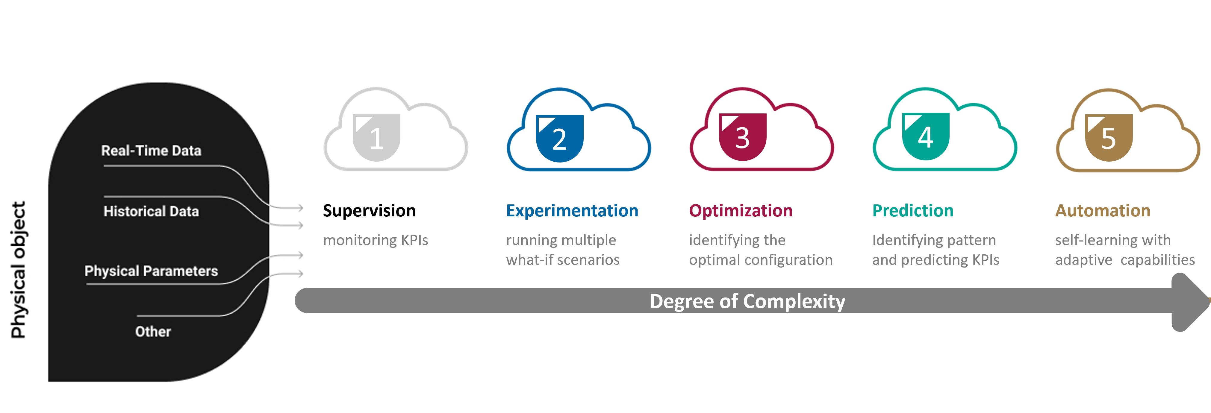
Figure 13.1: Evolutionary levels of digital twins in Industry 4.0.
Level 1: Supervision: This equips organizations with the capability to monitor their systems using simulation models, effectively tracking Key Performance Indicators (KPIs) and ensuring control over system performance. This phase unveils the potential to identify issues, bottlenecks, and deviations from expectations.
Level 2: Experimentation: Organizations utilize simulation models to run multiple what-if scenarios, gaining invaluable insights into how various variables impact system performance. This experimentation empowers decision-makers to refine their models, embracing the most desirable outcomes and KPI results.
Level 3: Optimization: As the digital twin journey progresses, the focus shifts to optimization. In situations with a plethora of scenarios or numerous decision variables, optimization models come to the forefront. These models enable the creation and testing of diverse scenarios, assisting organizations in identifying the optimal parameter combinations for their systems. Simio offers three different scenario selection and optimization tools (see Figure 13.2): Good Selection Procedure (GPS) and Kim and Nelson (KN) ranking and selection procedures, which attempt to identify optimal scenarios from a pre-defined set of alternatives. Additionally, it offers OptQuest, an optimizer for experiments. OptQuest functions as a black-box optimizer that optimizes a set of control parameters to obtain the best possible outcomes. It explores the solution space to iteratively refine the control settings, aiming to maximize or minimize a specified objective function.
Level 4: Prediction: The journey advances towards prediction. Well-designed simulation models yield high-quality synthetic data, enabling accurate forecasts of system behavior and patterns. Integration of predictive models like neural networks enhances the digital twin’s adaptability for informed decision-making in complex scenarios. Simio’s Neural Network tool is designed for implementing and fine-tuning these predictive models, ensuring precise prediction and intelligent decision-making in various industrial settings.
Level 5: Automation: At this stage, the system attains a level of maturity that enables self-adaptation and autonomous problem-solving. Reinforcement Learning (RL) modules integrated with simulation models facilitate this automation, allowing systems to make decisions in response to expected and unexpected events while minimizing disruptions. This level requires rigorous training and substantial data but aligns seamlessly with the data-rich environment of digital twin simulations.
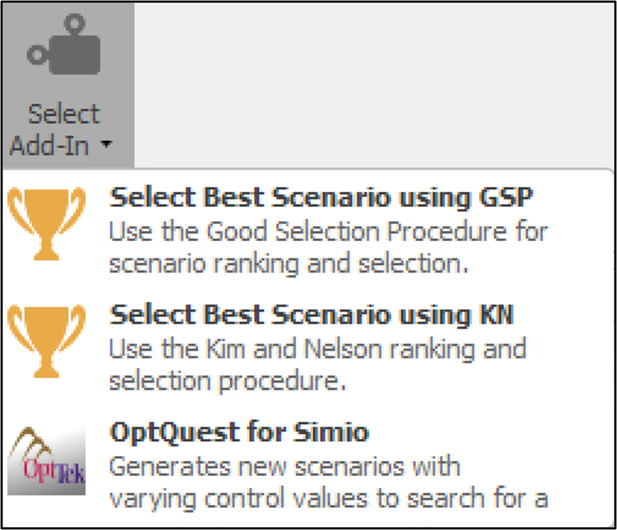
Figure 13.2: Optimization tools provided in Simio experiments.
13.2 Deep Learning Fundamentals
Deep learning, a subset of machine learning (ML) within the field of AI, draws inspiration from the human brain. Neural networks in deep learning mimic the way biological neurons propagate signals, reflecting the brain’s information processing strategies. As shown in Figure 13.3, in deep learning, neural networks consist of three main layers, each with a specific role in the learning and prediction process:
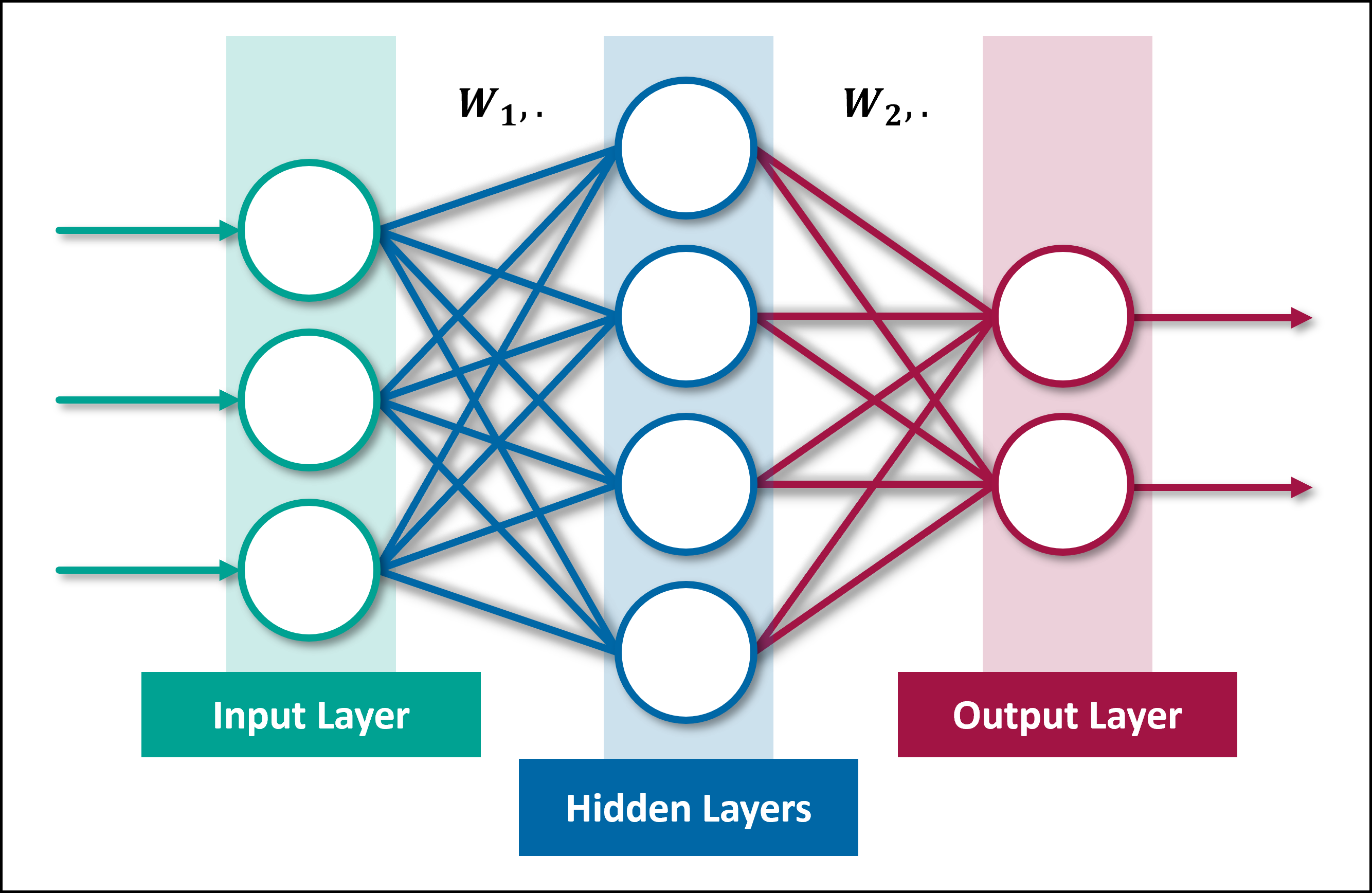
Figure 13.3: Structure of a Feedforward Neural Network with Input, Hidden, and Output Layers.
Input Layer: The input layer is the neural network’s initial stage, where raw data is received through units representing specific input features. It prepares and passes this data to subsequent layers, setting the foundation for learning.
Hidden Layers: The hidden layers, positioned between the input and output layers, is a fundamental component of neural networks. It can consist of multiple layers and nodes. The term “Deep” in deep learning refers to the presence of multiple hidden layers in a neural network.
Output Layer: The output layer is the final layer of a neural network, responsible for producing the network’s output. It transforms the information processed by the hidden layers into a format suitable for the specific task, such as classifying objects in an image or predicting numerical values.
These layers are connected in a feedforward manner, enabling the unidirectional flow of information from the input layer through the hidden layers and ultimately to the output layer. This sequential flow is precisely regulated by the connections between neurons, each characterized by a weight indicating the strength of the connection. The sign of a weight (- or +) also affects the output of the subsequent layer. Interactions between weights cause the transformation and propagation of signals through the layers. Smaller weight values represent milder effects, while larger weight values result in more pronounced impacts on the neural network’s output. The weights thereby control the strength of the connections between neurons and play a crucial role in determining how changes in input will influence the output.
As data progresses through the hidden layers, these weights guide the hierarchical transformation of features. At each layer, specific features are extracted and represented, with the weights (\(W\)) determining the significance of each component. This hierarchical feature extraction is a defining characteristic of deep neural networks, making them highly effective in tasks such as image recognition, natural language processing, and numerous other domains. Interested readers can refer to (Goodfellow, Bengio, and Courville 2016) for further insights into deep learning.
Suppose you aim to train a neural network to predict car prices based on specific input features. To accomplish this, you require data formatted with attribute values and corresponding prices across a large number of observations. This data is utilized to train the neural network by determining optimal weight. In this scenario, the input features could include parameters such as the car’s odometer reading, the number of cylinders it has, its miles per gallon (MPG), and other relevant attributes. The objective is to create a model using the neural network that, given these input features, can accurately predict the price of the car (see Figure 13.4). The neural network will then utilize its hidden layers and connection weights to learn patterns and relationships within the data. With each training iteration, the neural network adjusts its weights to minimize prediction errors and improve accuracy. Once the neural network is trained successfully, it can take new input data representing a car’s characteristics and use the trained model to make predictions about the car’s price.
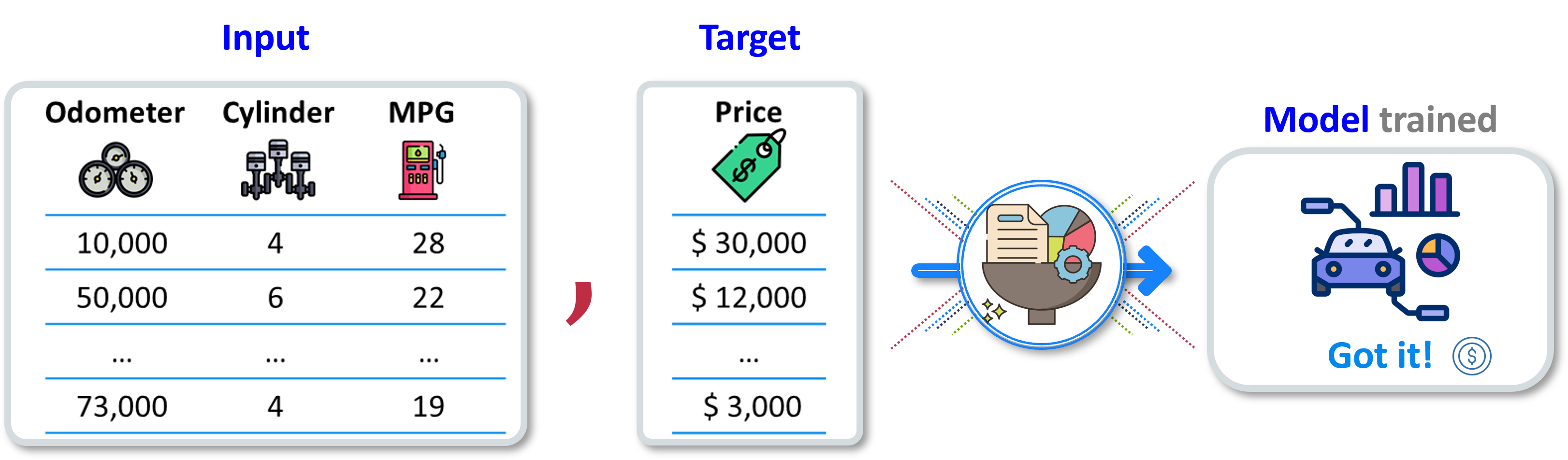
Figure 13.4: Input features for car pricing predictions using neural networks.
13.2.1 Simio Neural Network Tool
The integration of discrete event simulation and neural networks unlocks the full potential of prediction, allowing organizations to harness Level 4 capabilities in their digital twin implementations. This integration is highly complementary. The simulation model provides a robust framework for modeling complex systems, facilitating detailed analysis of processes and events. After verifying and validating the simulation model, it can generate abundant clean and labeled data for the studied system, effectively addressing the data-hungry nature of neural networks. In turn, neural networks can leverage the rich and well-structured data produced by simulations to develop a trained model and uncover system patterns.
This synergy enhances decision-making processes and offers several additional benefits. Once the training is complete, the trained model can be employed as a decision-making module in conjunction with the simulation run. This synergy enhances decision-making processes and offers several additional benefits, further optimizing processes and improving overall system performance.
Simio offers embedded support for neural networks, which includes the ability to utilize synthetic training data generated within the simulation environment. This feature allows for the rapid and cost-effective creation of training data, a process that could otherwise require significant time and resources to collect similar data from the factory floor. Additionally, Simio provides an interface for training the neural network model, enabling seamless integration of simulated data into the training process. These features offer several advantages to users:
Integrated Platform: Simio provides neural network modeling and simulation capabilities within a single platform, eliminating the need for external packages. Users can seamlessly integrate neural network capabilities into their simulation efforts without requiring additional software.
Code-Free: Simio simplifies the use of neural network tools, making them accessible without the need for coding. This code-free approach broadens the user base and facilitates neural network modeling. Simio’s Neural Network tool also includes essential optimizers for fine-tuning neural network parameters and weights, along with a graphical representation of training progress and neural network model accuracy.
Data Availability: Discrete event simulation packages like Simio excel at logging data on an event basis, offering a robust data source for training neural networks. Because neural network model performance is predicated on the quality of the training dataset, precise and thorough cultivation of input features is paramount. Discrete event simulation packages like Simio excel at logging data from any element of a system (entities, servers, queues, etc.), offering a limitless source of quality training data for neural networks. This is crucial since developers may need to add more features (data inputs) to their model for better performance. This allows users to collect any essential data from any element of the system (entities, servers, queues, overall systems, tallies, etc.) to meet their modeling needs hassle-free.
Efficient Data Collection: In the context of simulation modeling, data collection is rapid, risk-free, and efficient compared to real-world data collection methods. This efficiency enhances the training process for neural networks.
ONNX Compatibility: Simio supports ONNX (Open Neural Network Exchange), allowing users to import and export trained neural networks or other machine learning models. ONNX facilitates advanced training and promotes interoperability between different deep learning frameworks.
Performance Evaluation: Testing and evaluating the performance of trained models within Simio is a crucial step for further analysis. Simulation experiments conducted within virtual environments offer valuable insights into the performance of these models in scenarios closely resembling real-world situations. This approach enables users to validate the models before deployment, ensuring their effectiveness in practical applications.
It’s important to note that Simio’s implementation of neural networks follows a feedforward architecture, where data flows from the input neurons of the network to the output neurons without looping back to the input neurons. The current implementation only supports single outputs, which means that for multiple output prediction, multiple networks need to be trained and applied.
13.2.2 Step-wise Implementation of the Neural Network Tool
Utilizing the provided Neural Network tool in Simio can be accomplished in a few simple steps, ensuring a systematic approach to achieving accurate predictions and insights. This chapter presents both the implementation steps and a practical case study to illustrate the effective application of this tool within a simple manufacturing setting. The graphical representation in Figure 13.5 provides an overview of the key steps involved in using the Neural Network tool. These steps include creating a baseline model, collecting necessary data points, applying training modules, and conducting testing. Each step plays a significant role in the successful application of the Neural Network tool.

Figure 13.5: Illustration of the steps in the Neural Network tool: (1) Baseline model, (2) Data collection, (3) Training, and (4) Testing.
Step 1: Baseline Model: This step sets the foundation for the effective utilization of Neural Network tools. It focuses on developing the desired simulation model to lay the groundwork for further application of Neural Network models. In certain instances, additional adjustments and settings may be necessary to ensure that the model can collect the required data during the data collection phase.
Step 2: Data Collection: Once the baseline model is in place, users can leverage the data collection module of the Simio’s Neural Network tool. During this phase, the model collects the necessary data points according to specifications and stores them for future analysis.
Step 3: Training: With the required data in hand, proceed to apply the training module of the Neural Network tool. This phase involves integrating the collected data into a neural network structure and framework to unveil hidden patterns in the system. The outcome is a trained neural network predictor that can provide accurate predictions for the target object. The training model utilizes collected inputs and employs a feedforward neural network.
Step 4: Testing: Following the completion of training, the trained model undergoes testing to evaluate its performance. It is important to note that, similar to any modeling task, developing, training, and creating a high-performing model may require multiple iterations involving data collection, training, and testing. Initially, users may have limited insight into the data points and their relevance for training. Through iterative processes of data collection and training, the Neural Network model can be enhanced to achieve a satisfactory level of performance.
13.3 Example 13-1: Intelligent Dispatching with a Neural Network
This section offers a comprehensive walk-through of a case study that provides tutorials and clear instructions for the effective implementation and deployment of the Neural Network tool. The case study demonstrates the practical application of the tool within a simple manufacturing setting, illustrating a step-by-step process to achieve accurate predictions and insights. In this model, an “AI-driven approach” is introduced, where a trained neural network makes dispatching decisions. This approach relies on predictions of the expected completion time for each order at each workstation. Orders are routed to the workstation with the lowest predicted completion time, based on order characteristics, workstation status, and the overall system status. This advanced approach facilitates informed decision-making, moving beyond traditional methods like random or cyclic dispatching, or heuristic-based approaches (e.g., shortest processing time or shortest queue length).
13.3.1 Baseline Model: Manufacturing Environment
The applied intelligent approach introduced in this chapter is based on predictions generated by a neural network. This neural network predicts the expected completion time for each order at every workstation upon its arrival and subsequently directs the order to the workstation with the shortest predicted completion time. These predictions take into account various order characteristics, including processing times, order type, and the overall system state such as workstation status, among others. The Baseline model is shown in Figure 13.6.
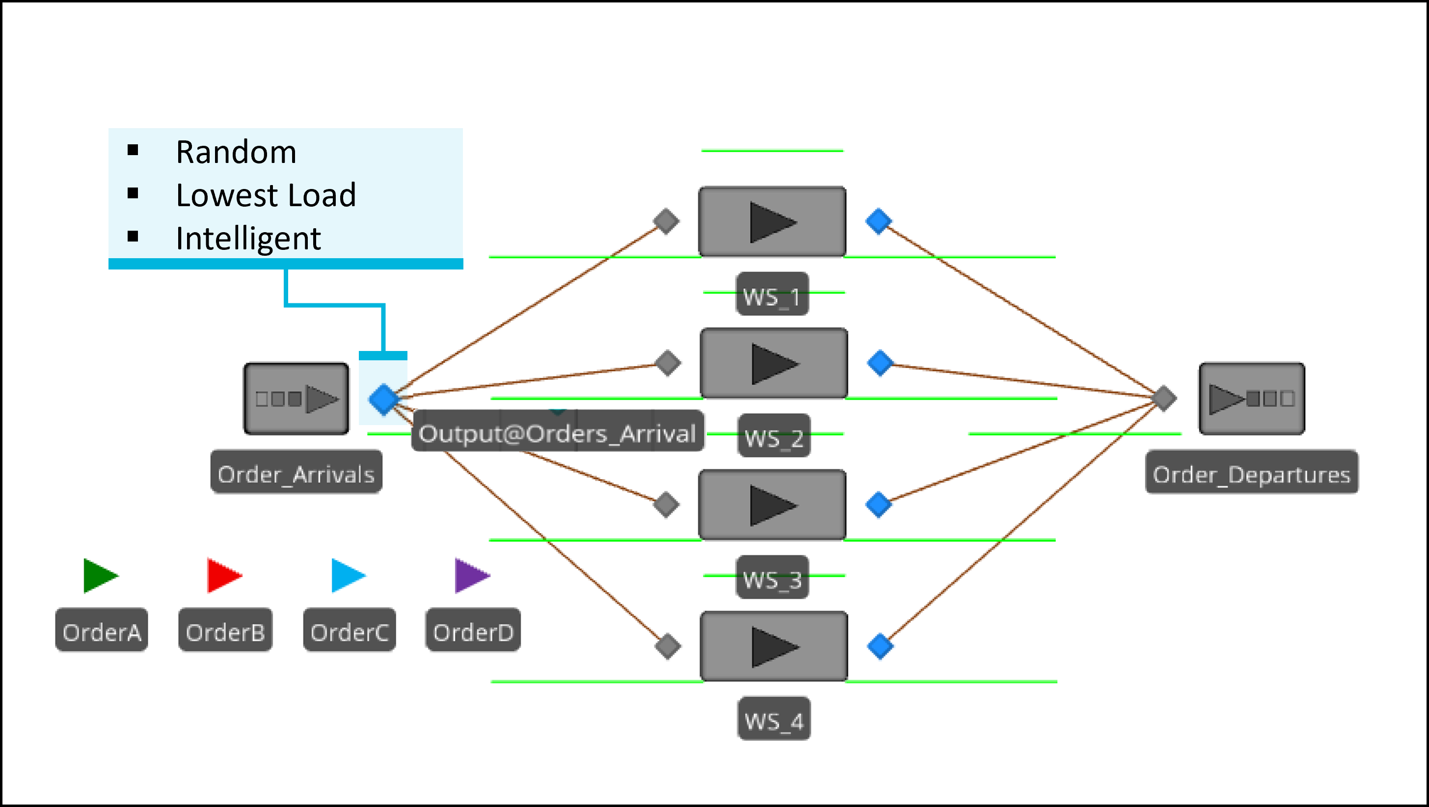
Figure 13.6: Simio model of the example manufacturing environment.
To analyze the effectiveness of this AI-enabled approach, this case examines two scenarios for dispatching orders to workstations:
Random Dispatching: Orders are assigned to workstations randomly.
Heuristic Dispatching: Orders are assigned to workstations with the lowest load (see Section 5.4).
Intelligent Dispatching: Neural Network-based dispatching based on predicted completion time.
Before delving into the details of the neural network model, an overview of the Baseline model implementation is provided to describe the model’s setting and configuration.
13.3.1.1 Source: Orders_Arrival
The orders creation is based on data from the tbl_OrderTypes
table, which defines the order mix: 40% for Order A, 15% for Order B,
25% for Order C, and 20% for Order D (Figure 13.7).
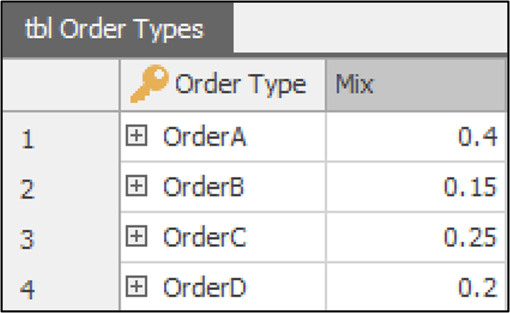
Figure 13.7: Order mix settings from the Order Types table.
The source utilizes these order mix probabilities to randomly generate
orders by setting the Table Row Referencing/Row Number property to
tbl_OrderTypes.OrderMix.RandomRow. This selects a random row from the
table based using the OrderMix values to determine probabilities and generates orders,
sending them into the system (Figure 13.8).
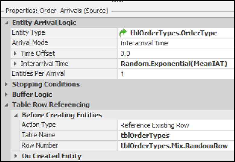
Figure 13.8: Orders Arrival Source object properties.
To adjust the arrival rate for experimental purposes, an exponential
distribution with an adaptable mean inter arrival time (meanIAT),
denoted as Random.Exponential(MeanIAT), is used. The initial mean IAT
is set to 4, indicating an average Inter Arrival Time (IAT) of 4
minutes, which corresponds to an average arrival rate of 15 orders per hour
(why?). A higher MeanIAT leads to fewer order arrivals, resulting in
reduced congestion, while a lower MeanIAT can potentially cause
congestion. This experimentation helps assess how different dispatching
rules perform under varying levels of model congestion. Refer to Figure 13.9 for the property setting.
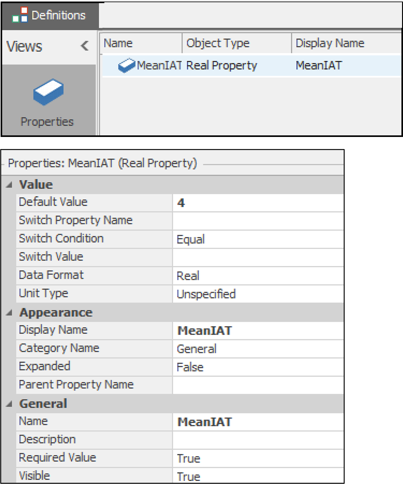
Figure 13.9: MeanIAT property definition.
13.3.1.2 Transfer Node: Output@Orders_Arrival
When an order is created, it is dispatched to one of the workstations
based on the implemented dispatching logic set at the Orders_Arrival
output node (Output@Orders_Arrival). To make the dispatching decision
dynamic, the Selection Goal property is set to a new referenced
property called Dispatching_Method (Figure 13.10).
This property allows dynamic goal selections including Smallest Distance, Largest Distance,
Preferred Order, Cyclic, Random, Smallest Value, and Largest Value.
Users can choose any of these dispatching approaches as part of the
experiment to compare their performance. The default selection rule is
‘Random.’
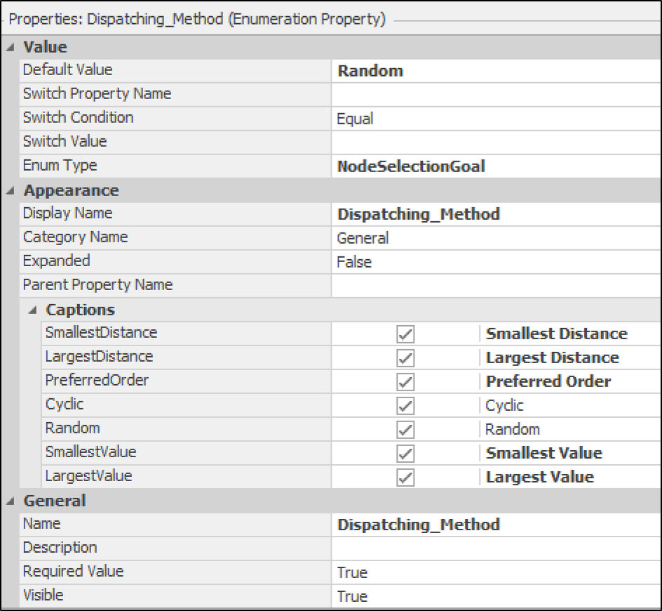
Figure 13.10: Dynamic dispatching options for flexible workstation assignment by setting a new referenced property, Dispatching Method.
This property is utilized as part of the dispatching approach on the
Output_OrdersArrival. As shown in Figure 13.11, the Entity Destination Type is set to
Select From List, indicating that orders are routed to a list of nodes
provided in a table called tbl_Node_List (Figure 13.12) containing all workstation input nodes for random or intelligent dispatching based on the specified Dispatching Method. The Transfer Node selects a workstation
based on the Selection Goal. The defined property, Dispatching_Method`, is referenced as the selection goal. Consequently, depending on the user’s selection, orders are routed to the servers. For
instance, consider these scenarios:
Random (Default): This option implements the Random Dispatching scenario. A workstation is randomly selected for each order for processing. All nodes have an equal probability (25%) as defined in the
RndSelectionWeightcolumn of thetbl_Node_Listtable. In this case, theSelection Expressionis not considered, and all orders are dispatched without prediction.Lowest Load: Orders are routed to workstations with the Smallest Value of load (in process, in route, and in queue). Refer to Chapter 5 for further details. The selection expression is set to
Candidate.Node.AssociatedStationLoad.Intelligent Dispatching: This option implements the Intelligent Dispatching scenario. When
Smallest Valueis selected, theSelection Expressionis utilized as a reference for evaluation. In this case, the expression is set toCompletionTimePredictor.PredictedValue(Candidate.Node.AssociatedObject).This indicates that the Transfer Node employs a trained neural network to predict the completion time of upcoming orders at each workstation and selects the workstation with the smallest completion time. This logic is applied after the Neural Network training is complete and produces satisfactory results. The term
Candidate.Node.AssociatedObjectrepresents all possible nodes listed intbl_Node_List, making the evaluation dynamic without requiring additional processes or logic. When an order (entity) reaches the output node, a token enumerates through the list of nodes (in this case, the input nodes of workstations) and uses the associated object (workstations) characteristics to determine the completion time.
This setup enables experiments to compare the base model (Random Dispatching) with the trained model (Intelligent Dispatching) to assess their performance.
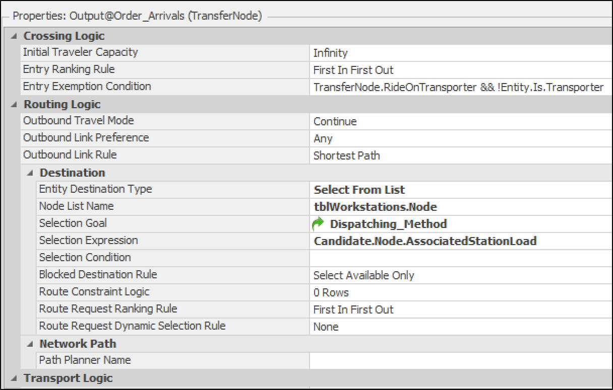
Figure 13.11: Routing orders to workstations: Output OrdersArrival property configuration.
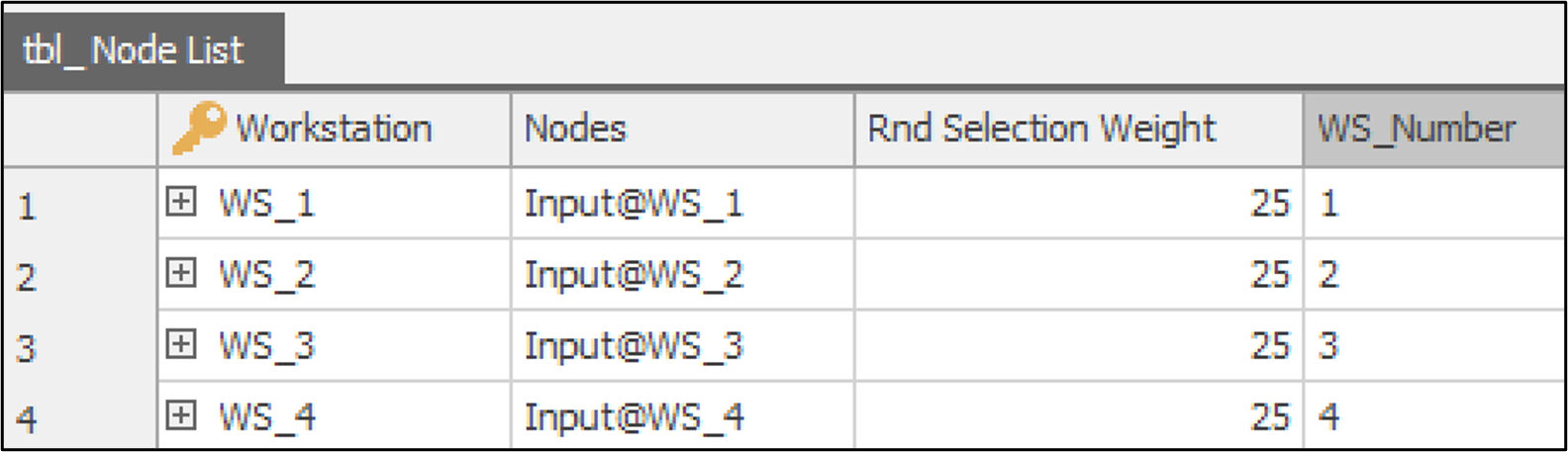
Figure 13.12: Node List table displaying workstation input nodes for order routing
This transfer node also has an state assignment and an add-on process,
Output_OrdersArrival_Exited, which is used to save the inputs for the
Neural Network. The details of this process will be discussed in Section
13.3.2.
13.3.1.3 Workstations: WS_1, WS_2, WS_3, and WS_4
Once an order is released, it will be dispatched to one of the
workstations in the model. These workstations operate in parallel, each
with a capacity of 1, and can process all types of orders. However, the
processing time for orders varies at each workstation. To facilitate
this implementation, a new table is designed, tbl_OrderDestination.
As illustrated in Figure 13.13, this table includes three columns:
OrderType, a foreign key property referring to the OrderType in the
tbl_OrderTypes table; Workstation, a foreign key property referring
to the Workstation in the tbl_NodeList table; and an Expression
Property, ProcessingTime, which specifies the processing time for
orders. This table contains 16 rows, each representing a unique
distribution for any order and workstation combination (\(4\) orders
\(\times\) \(4\) workstations). A mix of triangular distributions with
different minimum, mode, and maximum values, as well as uniform
distributions with (minimum, maximum) values, is used to define
processing times. These values are arbitrarily chosen. Therefore, an
effective dispatching rule should avoid assigning orders to workstations
with extended processing times and instead consider those with
reasonable processing times.
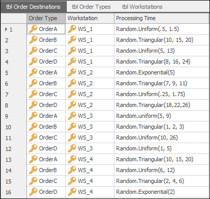
Figure 13.13: Order Destination table detailing order types, workstations, and processing times.
To set up the workstation, only the processing time and reliability logic need to be defined. An example property setting for one of the workstations is shown in Figure 13.14. The processing time expression (in minutes) is set to:
tbl_OrderDestination[1].ProcessingTime
which refers to the tbl_OrderDestination table to use the distribution
defined under its ProcessingTime to generate processing time. This
table cross-references the order type and workstation to select the
appropriate defined distribution to generate processing time. For
instance, if the order is Order B and the workstation is WS_1,
Random.Triangular(10,15,20) will be used to generate the processing
time.
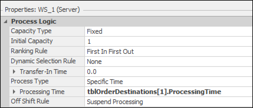
Figure 13.14: Property settings of WS 1; settings for other workstations are similar.
13.3.1.4 Sink: Orders_Exit
After finishing the process, orders leave the system from a sink, called
Orders_Exit. No additional settings are required. It needs to be noted
that all objects in the model are connected using connectors for
simplicity.
13.3.1.5 Initial Results
To test the base model, two dispatching methods were compared: 1) ‘Random’ and 2) ‘Smallest Value,’ considering the associated loads (Candidate.Node.AssociatedStationLoad). Both scenarios had a common mean inter-arrival rate (MeanIAT=4) for a fair comparison of the results.
The results show that the second scenario, with the smallest associated station load, outperformed the ‘Random’ approach by reducing the average Time in the System and the Number of Orders in the System (NIS). Additionally, it had varying impacts on the utilization rates across different workstations, indicating a more efficient distribution of workload among workstations (see Figure 13.15).

Figure 13.15: Comparison of Random and Smallest Vaue dispatching methods.
13.3.2 Data Collection: Generating Training Data
The quality of the data used for training a neural network is of utmost importance. The accuracy of the model is directly proportional to the quality of the training data. Therefore, it is crucial to ensure that the data is of high quality and quantity to achieve successful training of neural networks.
In the second step, it is necessary to determine which data points from the simulation model accurately mirror the dynamics of the system and can help achieve an accurate prediction. Depending on the training purpose, this can include data related to entities, servers, overall system measures, and many others.
The objective of this model is to predict the completion time of orders within each workstation. Therefore, the important data points that can help with this prediction can be:
Workstations’ Load: Indicates the number of orders currently loading the processing queue or waiting queue of each workstation.
Expected Processing Time: Calculates the expected processing time, a critical factor in determining completion time. This time represents the processing duration of an order at a workstation and is derived from a defined distribution.
Workstation Status: Specifies the operational state of the workstation, including whether it is
starved,processing, orfailedbased on the reliability logic. These data are essential for understanding the operational status of the workstation.Destination Workstation: Specifies the destination workstation to which the order will be routed.
To proceed with this modification, it is recommended to duplicate the initial base model and create a new model called NN_model (Figure 13.16).
As the model changes, the inputs might need to be tweaked to adjust to new information. In general, when selecting input data for a neural network, the approach is to list the information needed to create a closed-form estimate of the value being predicted and use that list as the inputs to the neural network. Using this approach, you might discover even more inputs that could be useful when predicting the completion time. Based on this introduction and data preprocessing, the setup instructions for ‘Data Gathering’ are as follows:
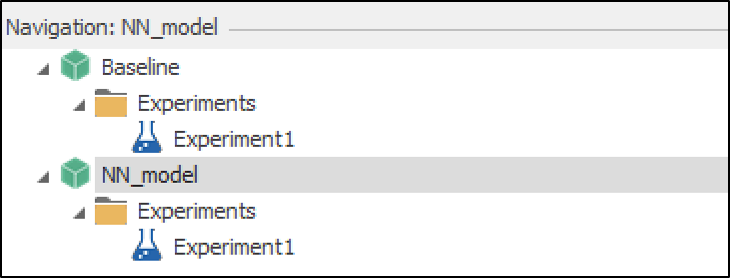
Figure 13.16: Creating a new model (NN Model) to apply the Neural Network tools.
13.3.2.1 Update Transfer Node: Output@Orders_Arrival
The initial settings of the Output@Orders_Arrival are discussed in
Section 13.3.1.2. To complement its data collection
part, some other changes need to be made:
- Define an Event: Create an event named
SaveInputsto be used as part of an add-on process for saving input data for neural network data collection (Figure 13.17).
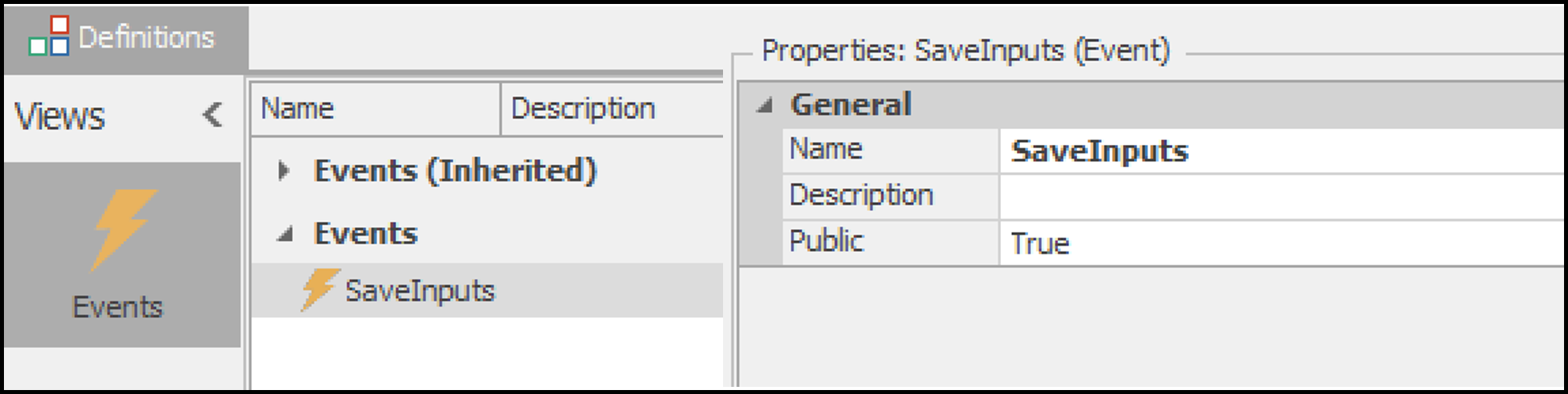
Figure 13.17: Defining the SaveInputs event.
- Define a State Variable: From the
Definitionstab, create a new Entity Reference State Variable namedCurrentOrder(Figure 13.18).
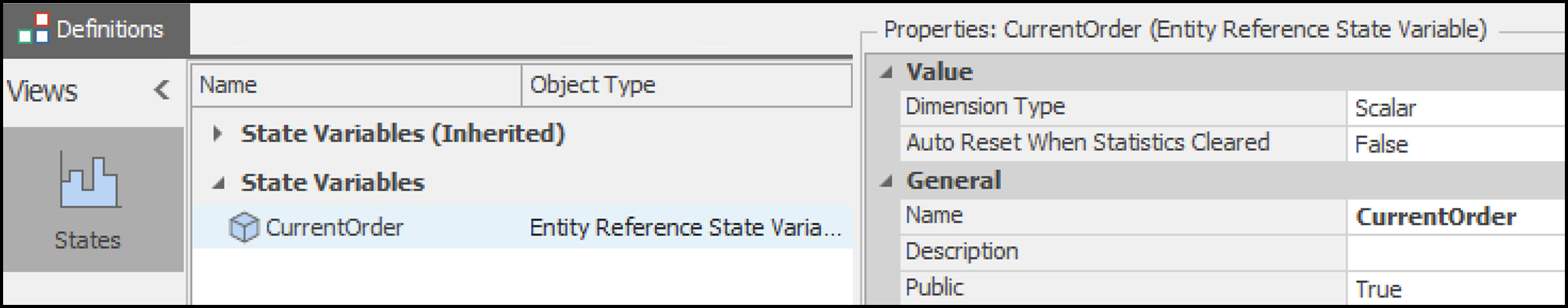
Figure 13.18: Defining CurrentOrder entity reference state variable.
- Set the State Assignment: In the scenario where the neural
network is trained, the TransferNode queries the neural network for
predictions before selecting the entity’s destination. Following
this, the single process within the model configures the entity’s
row in the
tbl_NodeList, assigns the current entity to the model’sCurrentOrderEntityReference state, and triggers the Save Inputs event. This event, in turn, prompts the Neural Network element to record input data. This modification enables additional streamlining, including the removal of redundant nodes, connectors, and state assignments (Figure 13.19).
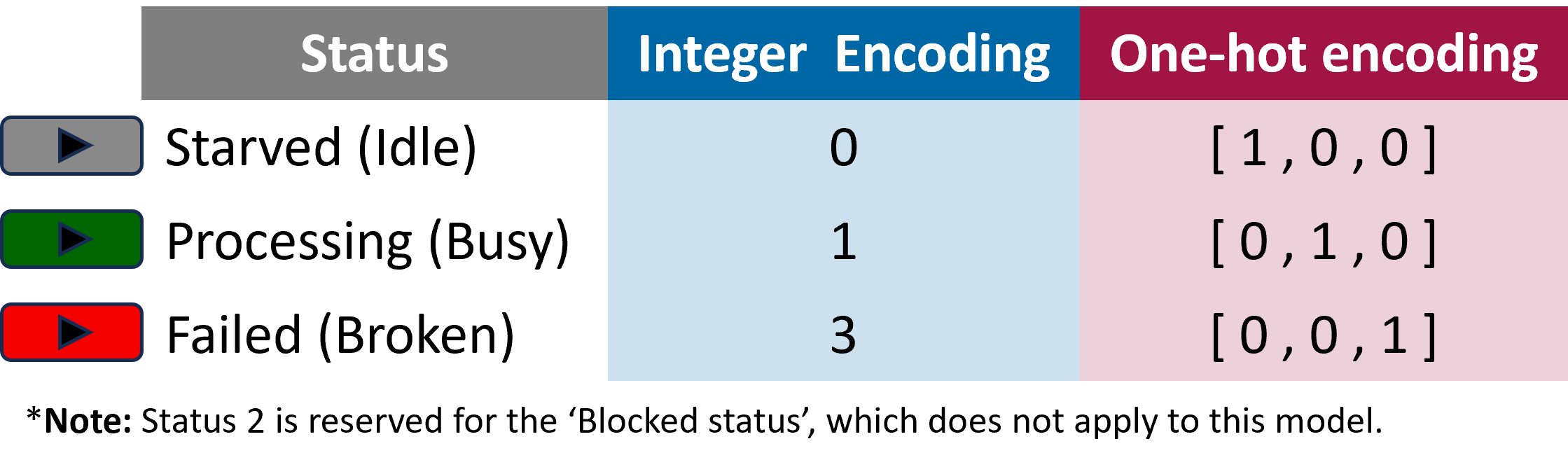
Figure 13.19: One-hot encoding of workstation status.
- Configure an Add-on Process: The add-on process is utilized in both trained and untrained neural network cases. In the trained scenario, after the TransferNode assigns the entity to a destination node, it’s essential to establish a row reference for the entity in the appropriate table. This ensures that when evaluating the Processing Time expression on the Server, the correct row is referenced. For the untrained case, the Assign step guarantees that the neural network input expressions can access the property entity reference, while the Fire step prompts the neural network element to record input data (Figure 13.20).
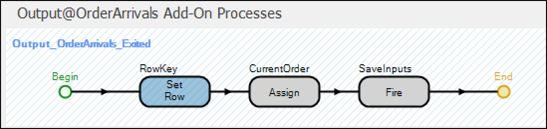
Figure 13.20: Configuration of TransferNode Output OrderArrivals Exited add-on process for efficient data handling.
13.3.2.2 Neural Network Model: CompletionTimePredictorModel
Integrating a Neural Network within Simio involves initiating a Neural Network Model. These features continue to be enhanced, which is a good reason to keep your Simio software up-to-date (Check Appendix C for updating guidelines). Users can create a variety
of neural network models to meet their particular needs. Specifically,
the model named CompletionTimePredictorModel is configured to forecast
the completion time of orders. The setup process for the neural network
model includes configuring the following properties:
- Creating a Neural Network Model: From the ‘Data’ view in Simio, access the ‘Neural Network Models’ section to add a new model. Select ‘Add Feedforward Neural Network Model’ (Figure 13.21) to initiate a fully-connected feedforward neural network regression model with a set number of numeric inputs and a single numeric output. This type of model can have several hidden layers, with the number of layers and nodes as adjustable hyperparameters determined before the training phase. The ‘tanh’ function is commonly used as the activation function for hidden layers, whereas the identity function is utilized for the output layer’s activation.
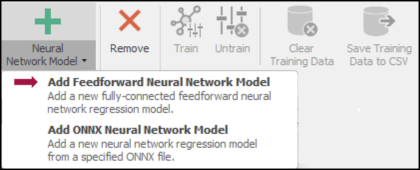
Figure 13.21: Creating a feedforward neural network model.
Setting the Model Properties: In this phase, initial properties including the model’s name, the number of input nodes, and the maximum size of the data repository are set (see Figure 13.22) . Further details, such as the configuration of hidden layers and model hyperparameters, are addressed during the training phase, Section 13.3.3.
Number Input Nodes:
9. The significance of this setting will be elaborated in Section 13.3.2.3, where the neural network element is defined.Maximum Records Limit:
5,000Name:
CompletionTimePredictorModel
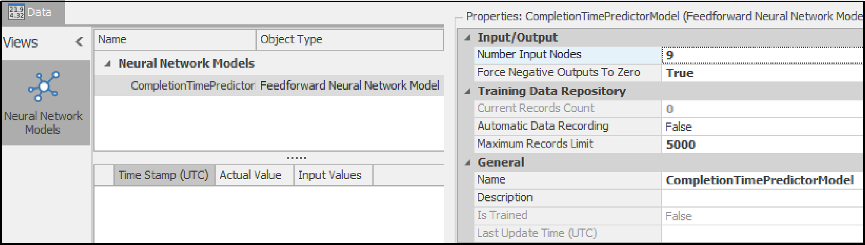
Figure 13.22: Setting the neural network model properties.
13.3.2.3 Element: CompletionTimePredictor
The Neural Network element in Simio is instrumental for integrating a
neural network-based model into the simulation’s decision-making
framework. The Input Value Expressions property of this element allows
for dynamic association of expressions with the model’s input layer.
When evaluation is needed during a simulation run, the element’s
PredictedValue function is utilized to perform a detailed evaluation
of the input expressions against a specific object in the simulation.
This leads to the neural network model processing these inputs to derive
an output value that serves to predict outcomes.
Creating a Neural Network Element: In the ‘Definitions’ tab of Simio, navigate to the ‘Elements’ view and select the ‘Data Science’ category to add a Neural Network Element.
Setting the Element Properties: Proper configuration of the neural network model is a fundamental step in ensuring its effectiveness and accuracy. It requires a meticulous definition of the expressions that represent the input data (independent variables), and the output data (dependent variable). Additionally, the model necessitates the setup of precise triggers for the consistent and reliable recording of data throughout its operation. The efficacy of the neural network’s performance is directly tied to the precision of these initial settings, underscoring the importance of this initial phase.
Basic Logic
Neural Network Model Name: Select the
CompletionTimePredictorModelfrom the predefined neural network models list.Input Value Expressions: Define the expressions that will generate the input values for the neural network model. These expressions represent the inputs discussed in Section 13.3.2. Figure 13.23 illustrates all the expressions used to record the model inputs. The first expression (a) captures the load on the associated workstation. The second set of expressions (b) employs one-hot encoding to log the workstation status as either
starved or idle (0),processing or busy (1), orfailed or broken (3). A set of four expressions (c) is utilized to log the workstation’s destination, again based on one-hot encoding. Finally, the last expression (d) records the expected processing time of the order at the workstation.Untrained Predicted Value Expression:
Random.Uniform(0, 1)Use this expression to provide a temporary predicted output value if the neural network model is not yet trained. This can also be used for debugging the trained model.
Training Data Recording
Save Inputs Triggers: Set to record a single row of input values. This suggests that there is an event-triggered action called "SaveInputs," which, when the defined event occurs, will trigger a process to save input data (Figure 13.24).
Save Actual Triggers: This expression captures the actual observed value when a ‘Save Actual’ trigger is activated. Here, the "Save Actual Trigger" is designed to save the actual observed values when a specific event, "Input@Orders_Exit.Entered" occurs (Figure 13.25).
Actual Value Expression: This expression captures the actual observed value when a ‘Save Actual’ trigger is activated. Here, the output variable (Actual value) is the completion time or time in the system for the order which is defined as
TimeNow - ModelEntity.TimeCreated
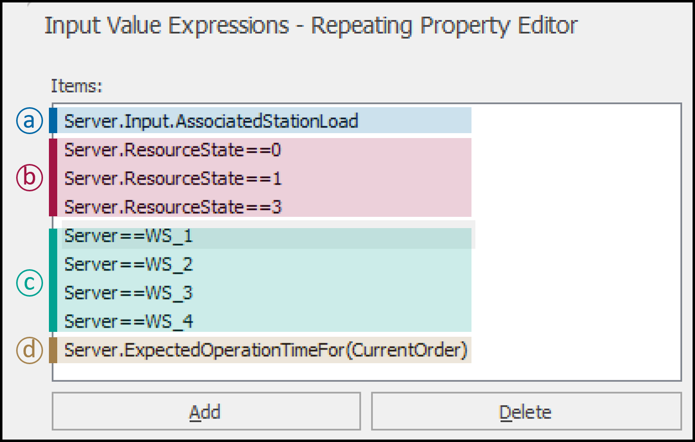
Figure 13.23: Input value expressions for the neural network element.
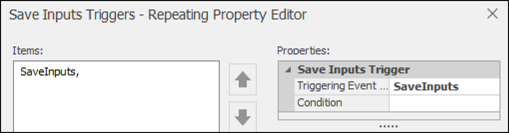
Figure 13.24: Save Inputs trigger using the event SaveInputs to save the input data.
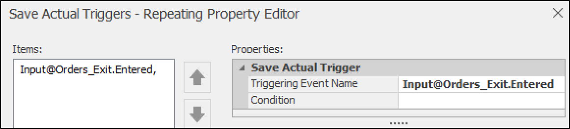
Figure 13.25: Save Actual trigger to save the output data (completion time).
Once all of the settings are complete, the simulation model is ready to
run and generate data points, storing them in the repository. From the
‘Data’ tab and the ‘Neural Network Models’ view, select the ‘Generate
Training Data’ tool. Click the “Run” button to begin the data collection
process. Simio will automatically run replications of the model until
the number of records in each neural network’s training data repository
equals the neural network’s Maximum Records Limit. In this case, the
neural network has the default Maximum Records Limit of 5,000. A neural
network model’s training records can be viewed by selecting the neural
network model. In Figure 13.26, the training data records for the
CompletionTimePredictorModel are visible. This includes ‘Time Stamp’,
the time data is recorded, ‘Actual Value’, and 9 input values as defined
in the Neural Network Element.
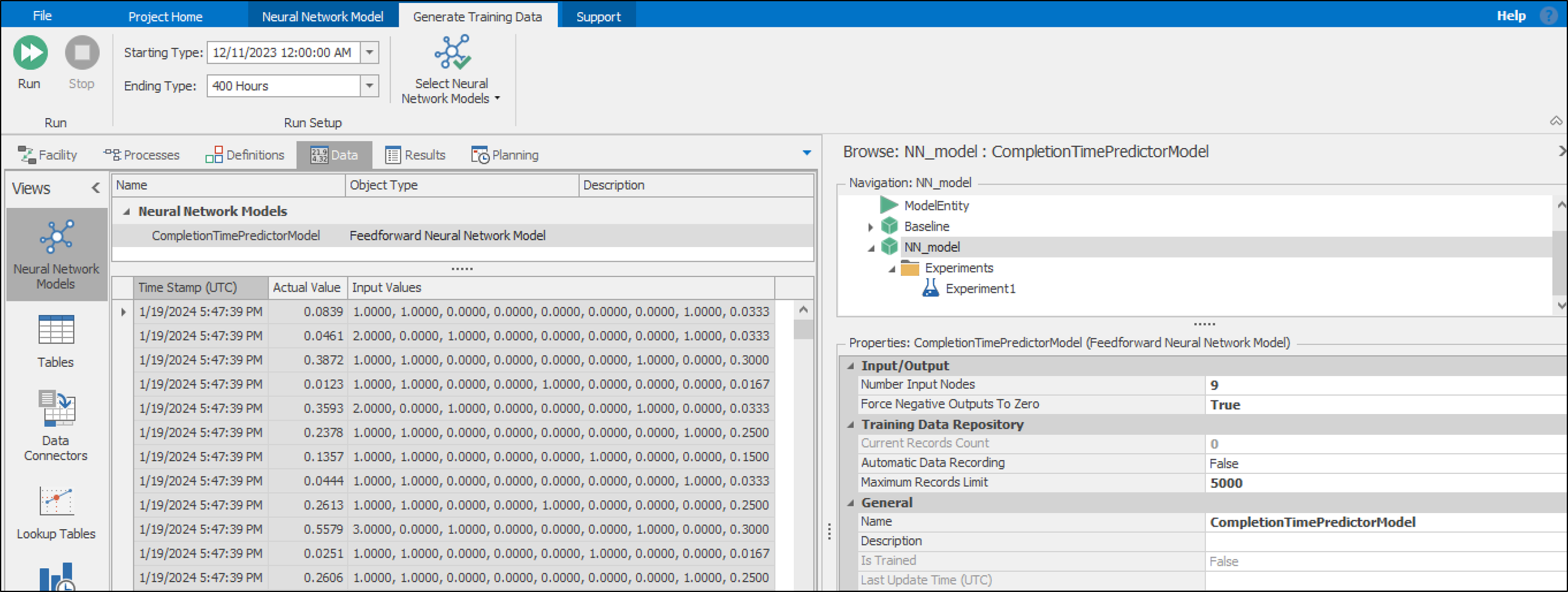
Figure 13.26: Generate Training Data tab of the Simio Neural Network tool.
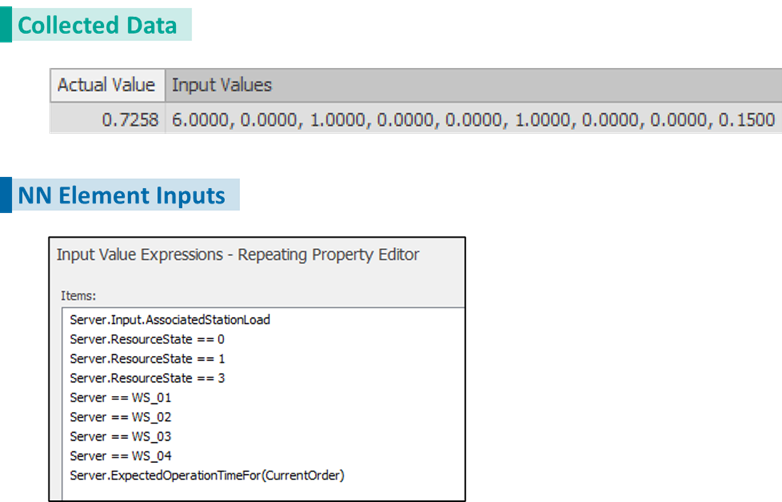
An interpretation of the first saved data is presented in Figure 13.27. As you may notice, the order of these numbers corresponds to the order in which the input expressions are defined in the ‘Input Value Expressions’ row of the element. The ‘Actual Value’ of 0.0839 represents the true completion time in hours, which the model aims to predict. The accompanying ‘Input Values’ are a set of binary encoded data points indicative of the operating conditions: two entries signaling the workload and status of a workstation, followed by three placeholders for workstation status, and another denoting the specific workstation ID (WS_4). The final numeric input, 0.0333, represents the expected processing time for the order. This structured data format allows the neural network to correlate various operational factors with the actual completion time, facilitating the development of a robust predictive model. When the required data are collected, the model is ready to start its training.
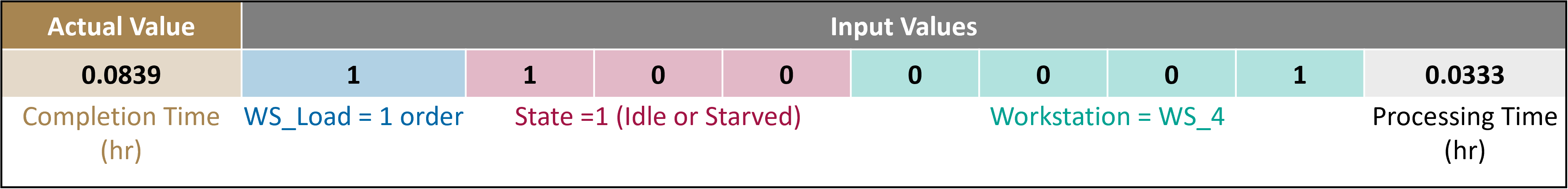
Figure 13.27: Interpretation of the saved data.
13.3.3 Training Process: Preparing the Model
Once high-quality data is collected, the next step is to effectively train the Neural Network Models using machine learning techniques. Simio provides a user-friendly interface for configuring and fine-tuning Neural Network Models. This includes defining the neural network’s architecture, learning rate, and optimizer type. Furthermore, the training progress can be monitored, and model performance can be evaluated to ensure it meets the desired accuracy and reliability criteria.
To start training, in the ‘Neural Network Models’ ribbon of the ‘Data’
tab, select CompletionTimePredictorModel and click ‘Train’ to open the
training dialog (Figure 13.28). The Train tool has the following
configuration options:
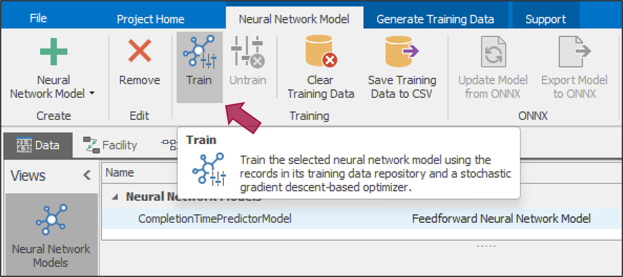
Figure 13.28: Training of the Neural Networks.
Data
Total Records Available: The entire dataset count available for training, validating, and testing the neural network.
Validation Holdout Percentage: The portion of the data reserved to get an unbiased estimate of the neural network’s performance during training.
Test Holdout Percentage: The portion of data set aside to evaluate the model’s performance after training, ensuring that it generalizes well to new, unseen data.
Network Architecture
- Number Hidden Nodes: The configuration of the neural network’s hidden layers, indicating how many nodes (neurons) are in each layer.
Training Algorithm
Max Epochs: The maximum number of complete passes through the entire training dataset before stopping the training process.
Optimizer Type: The optimization algorithm used to fit the neural network to the training dataset.
Learning Rate: Determines the step size for updating neural network parameters during training, influencing the convergence and speed of the optimization process.
Beta1 Parameter: A hyperparameter of certain optimization algorithms like Adam, controlling the exponential decay rate for the first moment estimates.
Beta2 Parameter: Another hyperparameter for optimization algorithms like Adam, this time controlling the exponential decay rate for the second-moment estimates.
Early Stopping Min Delta: The minimum change in the validation loss that qualifies as an improvement, used to decide when to stop training early.
Early Stopping Patience: The number of epochs to continue training without improvement in the validation loss before stopping early.
Progress Plot
- Skip First Epochs: An option to omit the initial epochs from the progress plot, potentially to avoid initial large-scale adjustments and focus on the finer training process.
To effectively utilize the Neural Network Training Tool, begin by selecting the appropriate number of hidden nodes and layers for the neural network. For a single hidden layer, specify the number of nodes (e.g., 9 for nine nodes). For multiple hidden layers, use a comma-separated list to define the nodes in each layer (e.g., 9, 4 for two layers with 9 and 4 nodes, respectively). Next, set the number of training epochs, representing how many times the neural network processes the entire training dataset. Keep in mind that the optimal number of epochs may vary and require experimentation.
Once the configuration is in place and the stage illustrated in Figure 13.29 is reached, initiate the training process while closely monitoring the epoch completion and any reported errors during training. This process allows for a better understanding of the network’s progress and facilitates necessary adjustments. During training, the tool calculates and displays the Mean Squared Error (MSE) for training, validation, and test datasets, providing insights into the model’s performance.
\[MSE = \frac{1}{n} \sum_{i=1}^{n} (Y_i - \hat{Y}_i)^2\]
where \(n\) is the number of observations, \(Y_i\) is the actual value of the target variable, and \(\hat{Y}_i\) is the predicted value from the model. The goal is to have an MSE as close to zero as possible, indicating that the model’s predictions are exactly equal to the true values. The training, validation, and test MSE values were close in magnitude, suggesting that the model’s predictions were consistent across both seen and unseen data, demonstrating good generalization without significant signs of overfitting.
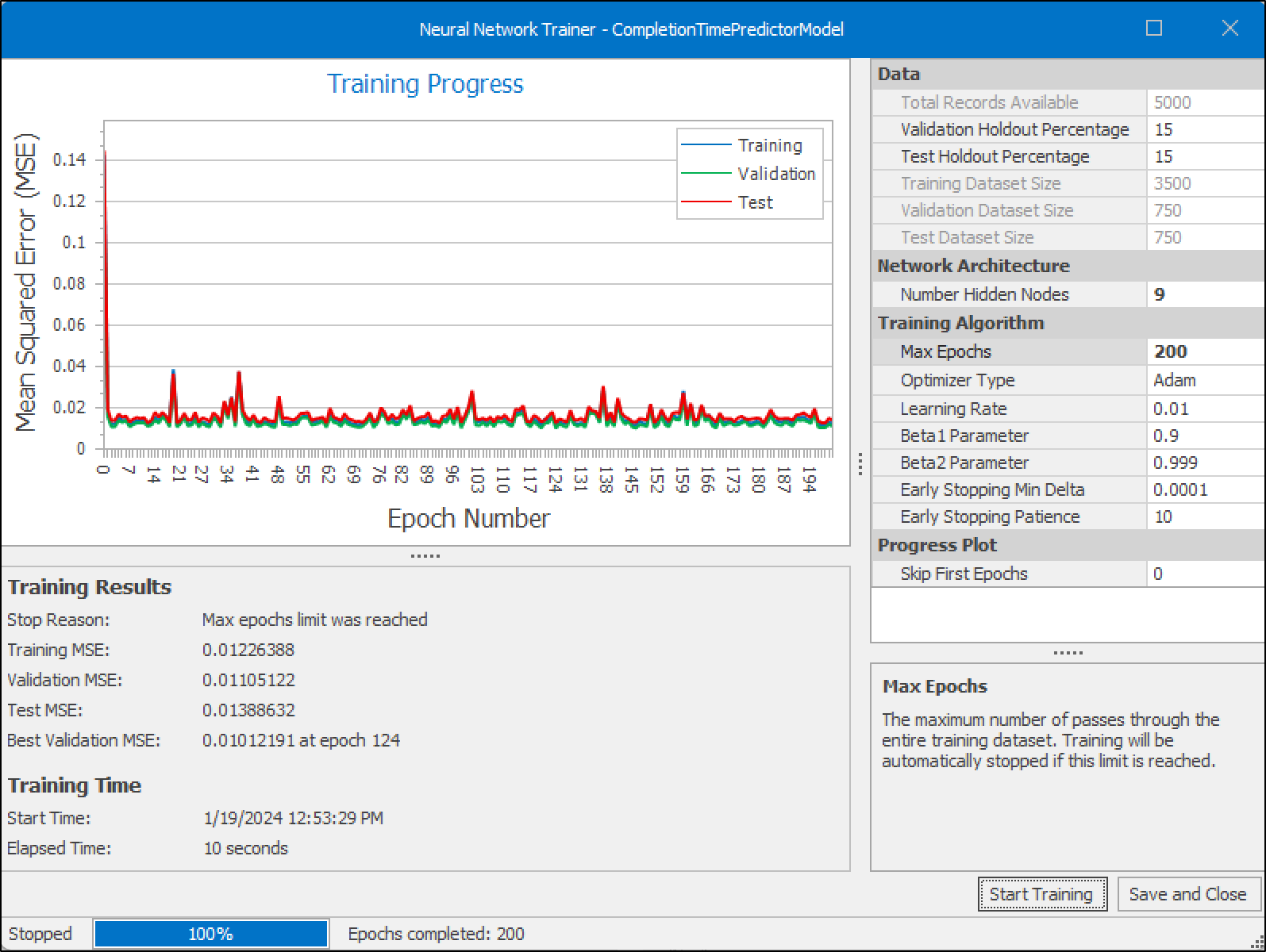
Figure 13.29: Neural Network Trainer displaying convergence of Mean Squared Error (MSE).
After the training process, save the neural network model when satisfied with its performance, ensuring it is fully trained and updated. With the training complete, you can now use the trained model to process new data and observe its performance, making the Neural Network Training Tool a powerful asset for your tasks.
13.4 Testing and Performance Evaluation
Once training is complete, the training status in the property window is
updated, with IsTrained set to True, and LastUpdateTime being
updated (Figure 13.30).
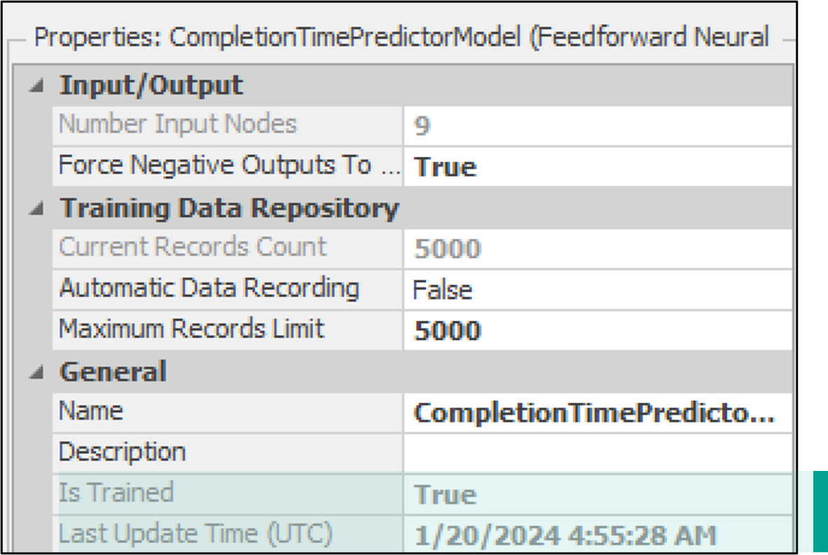
Figure 13.30: Training Status in the Property window.
To evaluate the neural network within the context of system performance, an experiment is used to compare the performance of the baseline model with a model containing the trained neural network. It is important to note that each time the neural network is trained, the experiment results may vary. Figure 13.31 illustrates the comparison between two models:
Lowest Load: The ‘Dispatching_Method’ is set to
Smallest Value, based on the Associated Load of workstations, representing a baseline scenario where orders are dispatched without specific logic or criteria. This serves as the control group for comparison.Intelligent Dispatching: The ‘Dispatching_Method’ is set to
SmallestValue, utilizing the neural network’s predictions to optimize order processing efficiency.
The results indicate that the Intelligent Dispatching method using the neural network predictor outperforms both the Random and Lowest Load strategies. As depicted in Figure 13.31, the trained neural network prediction model, when compared to the Lowest Load approach, exhibits a significant enhancement in operational efficiency. It effectively reduces the time spent in the system and the number of orders in the system. Unlike the relatively even distribution of tasks across workstations seen with the Lowest Load approach, the neural network model achieves a more targeted utilization, suggesting its predictive capabilities enable it to optimize workflow more effectively.
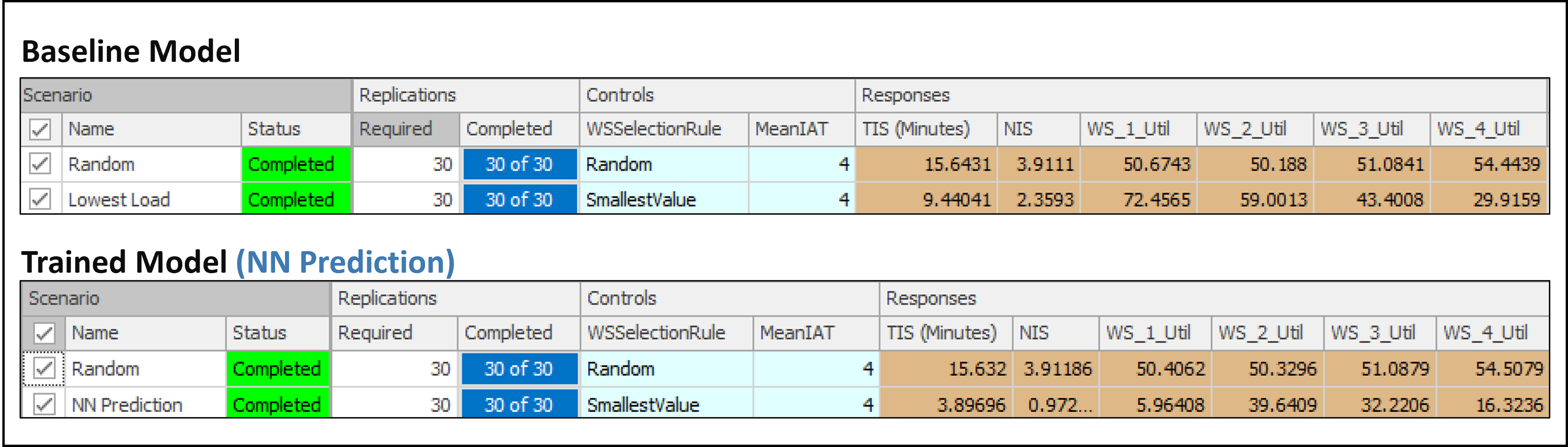
Figure 13.31: Performance comparison between Random, Lowest Load, and Intelligent dispatching using the trained neural network predictor.
13.5 Summary
Although AI has demonstrated many successes in multiple domains, its potential has not been fully leveraged for digital twin technology. The Simio Neural Network is a unique early tool for applying AI into digital twin platforms. Therefore, this chapter aims to introduce this tool, provide setup instructions, and discuss its applications.
The applicability of this tool is demonstrated in a manufacturing case study, where a neural network is trained to assist with dispatching four different orders among four parallel workstations (intelligent dispatching). In this example, each order has different processing times on each workstation, therefore, efficient dispatching requires considering multiple factors such as workstation loads and processing times. The Simio Neural Network tool is applied in two steps: (i) Data Collection, and (ii) Training. The first step enables users to collect data required for training the neural network. Once the adequate data is obtained, the training phase is executed to train the model for prediction. In this case, the prediction model was used to predict the completion time of orders on each workstation to enable the system to route orders to workstations with the shortest completion time. This predictor is trained based on important information regarding orders (order type) and workstation information (status, current load).
The performance of this Intelligent Dispatching is compared against two benchmarks: random dispatching and lowest load dispatching. The results show that if trained successfully, the intelligent approach can significantly optimize objectives, in this case, reducing the average time in the system.
This early example showcases the potential of AI in supporting digital twin technology for operational optimization, predictive analytics, and decision-making. It highlights the necessity of a thorough understanding and implementation process to fully exploit AI’s capabilities in this domain.
13.5.1 Iterative Refinement of the Neural Network model
Integrating neural network tools into digital twin technology is a dynamic and essential process for successful implementation. This integration requires regular model revisions, involving adjustments to logic, processes, variables, and attributes to ensure comprehensive data collection. For example, incorporating new orders into the model requires modifications to accurately reflect evolving dynamics. These adjustments maintain data relevance and precision, crucial for subsequent neural network retraining.
Following these revisions, a thorough data collection phase is initiated, reset, and repeated as needed to synchronize with the updated model parameters. This ensures the neural network is trained on the most current and relevant data.
The training phase itself involves iterative refinement of the neural network’s hyperparameters, including the neural network’s architecture, learning rate, or optimizer type. This iterative training optimizes the model’s performance, ensuring that the digital twin can provide precise predictions and insights for decision-making processes.
Through this iterative cycle of model revision, data collection, and training, neural networks progressively enhance their performance. This allows users to make more informed decisions and leverage the full potential of AI for their digital twin needs.
13.6 Problems
Discuss the main differences between using optimization tools like OptQuest and neural network modeling within a simulation environment such as Simio. Highlight the strengths and limitations of each approach and their appropriate use cases.
Explain the advantages of integrating AI, particularly neural networks, into digital twin models. How do AI-enabled digital twins enhance the capabilities of traditional digital twins?
Why is integrating neural networks with a simulation environment beneficial?
The figure below shows a snapshot of generated data during the data collection phase using Simio Neural Network tools. Use Figure 13.27 as a reference to decode Input Values (i.e., which server is used, what is the server status, etc.).
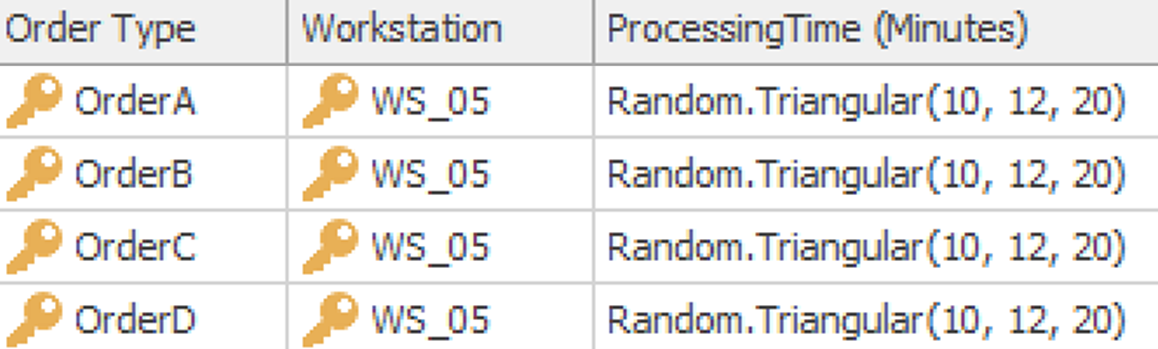
Consider Example 13.1 with the initial four workstations (WS_01, WS_02, WS_03, and WS_04). Now, consider adding a fifth workstation, WS_05, as a backup. WS_05 should be used when the predicted completion time for any of the primary workstations exceeds a certain threshold value, referred to as
CompletionThreshold. Implement a decision-making process within Simio using the Neural Network tool to route orders to WS_05 when the predicted completion time for WS_01 to WS_04 is greater thanCompletionThreshold. Analyze and visualize the performance of the system with this additional backup workstation. Steps:Add WS_05 to the model.
Update the ‘tblOrderDestinations’ table to include the processing time for all orders with WS_05.
Set the processing time for WS_05 to
tblOrderDestinations[1].ProcessingTime.Define a
CompletionThresholdproperty with the initial value of 20 minutes.Set MeanIAT to 2 to represent a more congested system.
Apply rerouting logic in Simio (Transfer node of Orders_Arrival - Output@Orders_Arrival) in such a way that orders are routed as explained. The changes should be applied to the “Value Expression” and “Selection Condition” of this node to implement the logic.
Test and validate the model to ensure it works as expected.
Run and experiment with different values of
CompletionThreshold(20 min, 50 min, and 100 min) and compare the utilization of all 5 workstations as well as TIS and NIS. Draw your conclusions.
In machine learning, plotting predicted values against actual values is important because it provides a visual representation of the model’s performance, making it easier to identify patterns, trends, and outliers. This visualization helps in quickly assessing the accuracy of the model; if the points closely align along the line \(y = x\), it indicates high predictive accuracy. Conversely, significant deviations from this line highlight areas where the model is underperforming, guiding necessary adjustments and refinements.
Simio Neural Network tool allows users to Save Training Data to CSV files, which enables further analysis of the data. Therefore, download this data and convert the file to an Excel format to visualize a dot plot of ActualValue vs. PredictedValue. What are your observations and conclusions based on this visualization?
Steps:
In Example 13-1 (NN Model), export the trained data from Simio as a CSV file using the “Save Training Data to CSV” option.
Open the exported CSV file in Excel.
Save the file in the Excel format (.xlsx).
Create a dot plot with ActualValue on the x-axis and PredictedValue on the y-axis.
Analyze the plot to identify patterns, trends, and deviations.
Draw conclusions about the model’s accuracy and performance based on the visualization.