Simio and Simulation: Modeling, Analysis, Applications - 7th Edition
Chapter 9 Advanced Modeling With Simio
The goal of this chapter is to discuss several advanced Simio modeling concepts not covered in the previous four chapters. The chapter is comprised of three separate models, each of which demonstrates one or more advanced concept. One common thread throughout the chapter is the comprehensive experimentation and use of simulation-based optimization with the OptQuest add-in. In Section 9.1 we revisit the Emergency Department model originally introduced in Chapter 8 and focus on the decision-making aspects of the problem. As part of the decision-making function, we develop a single total cost metric and use the metric to evaluate alternative system configurations. In this section, we also introduce the use of the OptQuest simulation-based optimization add-in and illustrate how to use this add-in. In Section 9.2 we introduce a Pizza Take-out restaurant model and incorporate a Worker object to demonstrate a pooled resource system. We then use the model to evaluate several alternative resource allocations, first using a manually-defined experiment, and then using OptQuest to seek optimal resource levels. Finally, in Section 9.3, we develop a model of an assembly line with finite capacity buffers between stations and demonstrate how to set up an experiment that estimates line throughput for different buffer allocations. Of course there are many, many advanced features/concepts that we are not able to discuss here so this chapter should be considered as a starting point for your advanced studies. Many other simulation and Simio-specific concepts are demonstrated in Simio’s SimBits and in other venues such as the proceedings of the annual Winter Simulation Conference (www.wintersim.org) and other simulation-related conferences.
9.1 Model 9-1: ED Model Revisited
In Section 8.2.7 we added hospital staff to our Emergency Department (ED) model and incorporated entity transportation and animation (Model 8-3). However, we didn’t account for the actual patient treatment and we didn’t perform any experimentation with the model at that time. Our goal for this section is to demonstrate how to modify Model 8-3 primarily to support decision making. Specifically, we are interested in using the model to help make resource allocation and staffing decisions. While we could have extended Model 8-3 by adding the patient treatment and performance metric components to that model, we chose to create an abstract version of the model by removing the worker objects and transportation paths and using Connector objects to facilitate entity flow. Our motivation for this was two fold: First, the abstract model is smaller and easier to present in the book; and second, to reinforce the notion that the “best” simulation model for a project is the simplest model that meets the needs of the project. In Model 8-3, our goal was to demonstrate the transportation and animation aspects of Simio incorporating Standard Library Worker objects. For Model 9-1, our goal is to demonstrate a model that can be used for decision-making and to demonstrate simulation-based optimization using Simio.
Figure 9.1 shows the facility view of Model 9-1. Note that the model retains the four patient entity objects (Routine, Moderate, Severe, and Urgent) along with SignIn, Registration, ExamRooms, TraumaRooms, and TreatmentRooms server objects. The Nurse and Aide Worker objects have been replaced with Doctor and Nurse Resource objects. Also, the transportation networks and Path objects have been replaced with a simplified network using Connector objects and the animation symbols for the patient entities and various rooms have been removed, as we are not primarily interested in modeling the physical patient movement (and because we wanted to simplify the model).

Figure 9.1: Facility view of Model 9-1.
Model 9-1 maintains the same basic problem structure where patients of four basic types arrive and follow different paths through the system using a Sequence Table to specify their routes. The only difference in the patient routing is that Urgent patients now exit through the NormalExit object whereas in Model 8-3 they exited through the TraumaExit object. Figure 9.2 shows the updated PatientData data table and Treatment Sequences table for Model 9-1. Note that the Escort Type column has been removed from the Treatments table and a Waiting Time column has been added to the PatientData table. As part of our resource allocation model, we track patient waiting time — defined as any time that the patient is waiting to see a doctor or nurse (including the interval from when the patient first arrives to when they first see a doctor or nurse). We will use the waiting time to determine patient service level and to balance the desire to minimize the resource and staffing costs. The Waiting Time entries in the PatientData table allow us to track waiting time by patient type using Tally Statistics. We removed the Escort Type column as we are no longer modeling the physical movement of patients and staff. For Model 9-1, we will not use the Computer Adjustment that we used for Registration process in Models 7-5 and 8-3 — instead, we will just use Treatments.ServiceTime column for the Server Processing Time property as we do with the other Servers.
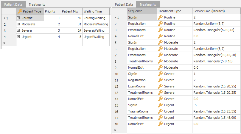
Figure 9.2: PatientData and Treatment data tables for Model 9-1.
In addition to the ExamRooms, TreatmentRooms, and TraumaRooms resources, Model 9-1 also incorporates the resource requirements for the patient examination and treatment (Model 8-3 used Nurse and Aide Worker objects to escort patients, but didn’t explicitly model the treatment of patients once they arrived at the respective rooms). The exam/treatment requirements are given in Table 9.1.
| Room | Exam/Treatment Resource(s) Required |
|---|---|
| Exam Room | Doctor or Nurse, doctor preferred |
| Treatment Room | Doctor and Nurse |
| Trauma Room | Doctor and Nurse or Doctor, nurse preferred |
When a patient arrives to a particular room (as specified in the Sequence table), the patient will seize the Doctor and/or Nurse resource(s) required for treatment. If the resources aren’t available, the patient will wait in the respective room until the resources are available (much as it works in a real emergency room!). As such, we separate the physical room resources (modeled using Server objects) from the exam/treatment resources (modeled as Resource objects) so that we can evaluate system configurations with different numbers of each – think of a typical doctor’s office that has more exam/treatment rooms that it has doctors.
As one would expect in an emergency room, priority for the Doctor and Nurse resources should be based on the priority level specified in the PatientData table (as we did in Model 8-3). So, for example if there are Routine and Moderate patients waiting for a doctor and an Urgent patient arrives, the Urgent patient should move to the front of the queue waiting for the doctor. Similarly, if there are only Routine patients waiting and a Severe or Moderate patient arrives, that patient should also move to the front of the doctor queue. We can implement this using the RankingRule property for the Doctor and Nurse resources. Figure 9.3 shows the properties for the Doctor resource. Setting the Ranking Rule property to Largest Value First and the Ranking Expression property to PatientData.Priority tells Simio to order (or rank) the queue of entities waiting for the resource based on the value stored in the PatientData.Priority field . One might also consider allowing Urgent patients to preempt a doctor or nurse from a Routine patient, but we will leave this as an exercise for the reader.
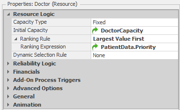
Figure 9.3: Properties for the Doctor resource.
In order to model the allocation of exam/treatment resources to patients, we will use Add-on Processes (see Section 5.1.4.1) associated with the respective room resources. Recall that Add-on processes provide a mechanism to supplement the logic in existing Simio objects. In the current model, we need to add some logic so that when a patient arrives in a room (exam, treatment, or trauma), the doctor and/or nurse who will provide the treatment are “called” and the patient will wait in the room until the “treatment resources” arrive. The current Server object logic that we have seen handles the allocation of room capacity, but not the treatment resources. As such, we will add-on a process that calls the treatment resource(s) once the room is available.
Figure 9.4 shows the two add-on processes for the ExamRooms object. The process ExamRooms_Processing is executed when an entity has been allocated server capacity (the ExamRooms Server) and is about to start processing and the ExamRooms_AfterProcessing add-on process is executed when an entity has completed processing and is about to release the server capacity.
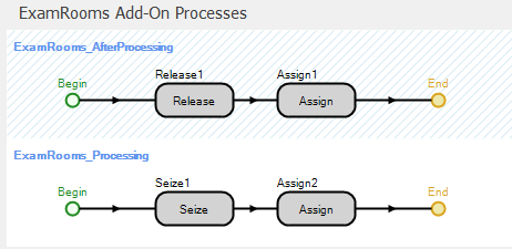
Figure 9.4: Add-on processes for the ExamRooms object.
When a patient enters the ExamRooms server, we do two things — seize the exam/treatment resource and record the waiting time once the resource is allocated to the patient. As shown in Table 9.1, patients in the exam room need either a doctor or a nurse, with the preference being a doctor if both are available. In Section 8.2.7.3 we demonstrated how to use Simio Lists and the PreferredOrder option for an entity to select from multiple alternatives with a preferred order. We use that same mechanism here — we defined a list (DoctorNurse) that includes the Doctor and Nurse objects (with the Doctor objects being first in the list) and seize a resource from this list in the Seize step in the add-on process. Figure 9.5 shows the DoctorNurse list and the details of the Seize step. Note that we specified the Preferred Order for the Selection Goal property so that the Doctor will have higher priority to be selected. Note that we could also have used the Server object’s Secondary Resources properties to achieve this same functionality, but wanted to explicitly discuss how these secondary resource allocations work “under the hood.”
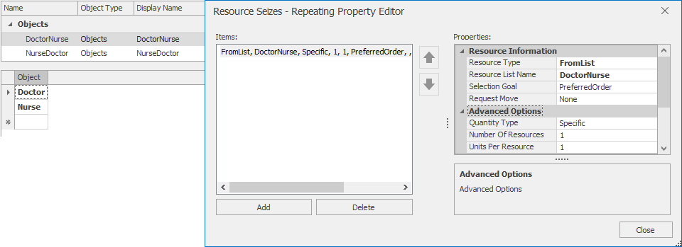
Figure 9.5: List and Seize details for the ExamRooms add-on process.
The Assign step, Assign2 is used to record the initial component of the patient waiting time and the Assign step, Assign1 is used to mark the time that the patient leaves the Exam room (more on this later). The Assign2 step will execute when the doctor or nurse resource has been allocated to the entity. Recall that we would like to track all of the time that a given patient waits for a doctor or a nurse. Since patients can potentially wait in multiple locations, we will use an entity state (ModelEntity.WaitingTime) to accumulate the total waiting time for each patient. The WaitingTime and tmp (see below) entity states are both type Real so that they record decimal hours in simulation time (the default units for TimeNow). Figure 9.6 shows the properties for the the two Assign steps.
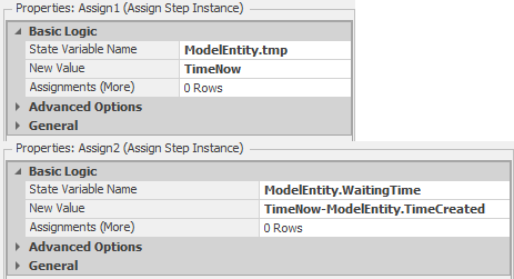
Figure 9.6: Assign step properties.
In Assign2 we are assigning the value TimeNow-ModelEntity.TimeCreated to the state ModelEntity.WaitingTime. This step subtracts the time that the entity was created (the time the patient arrived) from the current simulation time (stored in the model state TimeNow) and assigns the value to the entity state ModelEntity.WaitingTime. If the entity represents a Routine patient, this will be the total waiting time for the patient. Otherwise, we will also track the time the patient waits after arriving to the TreatmentRooms. In order to track this additional waiting time Assign1 marks the entity — stores the current simulation time to the entity state ModelEntity.tmp. We will use this time when the entity arrives to the Treatment room and is allocated the necessary resources. The Release step in the ExamRooms_Processed step releases the doctor or nurse resource seized in the previous process.
Figure 9.7 shows the add-on processes for the TraumaRooms object. The processes are similar those for the ExamRooms object. The only difference is that the TraumaRooms_Processing process includes two seize steps — one to seize a Doctor object and one to seize a Nurse object or a Doctor object. Since our preference is to have a nurse in addition to the doctor rather than two doctors, we seize from a list named NurseDoctor that has the Nurse objects listed ahead of the Doctor objects (the opposite order from the DoctorNurse list shown in Figure 9.5 and used in the ExamRooms object). Note that the Release step (Release2) specifies both resources that need to be released after processing.

Figure 9.7: Add-on processes for the TraumaRooms object.
Figure 9.8 shows the add-on processes for the TreatmentRooms object. Patients come to the treatment from either the trauma room (Urgent patients) or from the exam room (Moderate and Severe patients) so we cannot use the entity creation time to track the patient waiting time (as we did before). Instead, we use the previously stored time (ModelEntity.tmp) and use a second Assign immediately after the Seize in order to add the waiting time in the treatment room to the patient’s total waiting time (recall that an entity (technically, it’s a token that waits at the Seize step, but the token represents the entity) remains in the Seize step until the resource is available — the queue time).
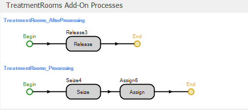
Figure 9.8: Add-on processes for the TreatmentRooms object.
In this process we use a single Seize step to seize both required resources rather than using separate Seize steps as we did previously in the TraumaRooms_Processing process. Figure 9.9 shows the properties and Repeat Group for the Seize step. Note that we use these two different methods for demonstration purposes only — we could easily have used a single step or two steps in both processes.

Figure 9.9: Seize4 step with two resource seizes
Figure 9.10 shows the properties for the Assign step in the TreatmentRooms_Processing add-on process. The basic concept of marking an entity with the simulation time at one point in the model, then recording the time interval between the marked time and the later time in a tally statistic, is quite common in situations where we want to record a time interval as a performance metric. While Simio and other simulation packages can easily track some intervals (e.g., the interval between when an entity is created and when it is destroyed), the package has no way to know which intervals will be important for a specific problem. As such, you definitely want to know how to tell the model to track these types of user-defined statistics yourself.
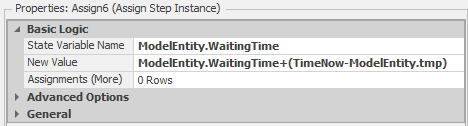
Figure 9.10: Assign step properties for adding the second entity wait component.
Figure 9.11 shows the add-on processes for the NormalExit object. When a patient leaves the system, we will update our waiting time statistics that we will use in our resource allocation analysis.
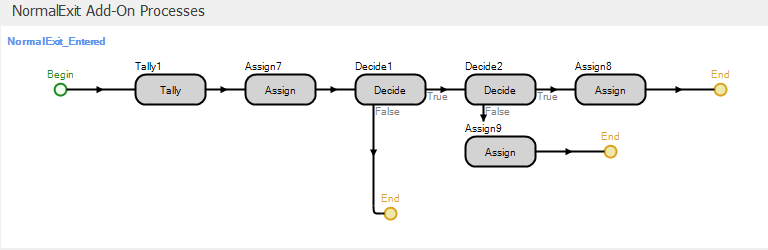
Figure 9.11: Add-on processes for the NormalExit object.
The Tally step (see Figure 9.12 for the properties) records the waiting time for the patient (stored in the WaitingTime entity state).
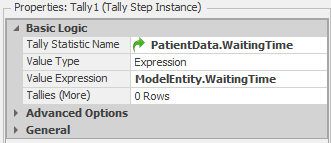
Figure 9.12: Tally step properties.
The PatientData.WaitingTime value for the TallyStatisticName property indicates that the observation should be recorded in the tally statistic object specified in the WaitingTime column of the PatientData table (Figure 9.2 shows the data tables and Figure 9.13 shows the tally and output statistics for the model). As such, the waiting times will be tallied by patient type. This is another example of the power of Simio data tables — Simio will look up the tally statistic in the table for us and, more importantly, if we add patient types in the future, the reference does not need to be updated. The Assign step adds the waiting time for the entity (stored in the WaitingTime entity state) to model state TotalWait so that we can easily track the total waiting time for all entities.
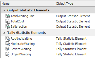
Figure 9.13: Model Elements for Model 9-1.
The final set of steps in the process are used to track the patient service level. For our ED example, we define service level as the proportion of Routine patients whose total waiting time is less than one-half hour (note that we arbitrarily chose one half hour for the default value). So the first thing we need to do is identify the Routine patients — the first Decide step does this (see Figure 9.14 for the step properties).
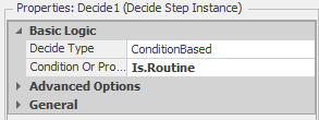
Figure 9.14: Decide step properties for identifying Routine patient objects.
Next, we need to determine if the current patient is “satisfied” based on that patient’s waiting time. The second Decide step does this (see Figure 9.15 for the step properties).
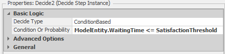
Figure 9.15: Decide step properties for determining whether the patient is satisfied based on waiting time.
Note that we used a referenced property (SatisfactionThreshold) rather than a fixed value (0.5 for one-half hour) to simplify the experimentation with different threshold values. If the patient is satisfied, we increment a model state for counting satisfied customers (SatisfiedRoutine). Otherwise, we increment a model state for counting unsatisfied customers (UnsatisfiedRoutine). The two Assign steps do this. We will use an output statistic to compute the overall service level for a run. Figure 9.13 shows the model output statistics and Figure 9.16 shows the properties for the Satisfaction output statistic where we compute the proportion of satisfied patients.
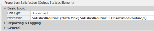
Figure 9.16: Properties for the Satisfaction output statistic.
Finally, we will use several referenced properties to support our resource allocation analysis. Since we are interested in determining the numbers of exam, treatment, and trauma rooms and the numbers of doctors and nurses required in the Emergency Department, we defined referenced properties for each of these items. Figure 9.17 shows the model properties and Figure 9.3 shows how the DoctorCapacity property is used to specify the initial capacity for the Doctor resource. We specified the Nurse object capacity and ExamRooms, TreatmentRooms, and TraumaRooms server object capacities similarly.
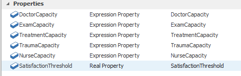
Figure 9.17: Model properties for Model 9-1.
Figure 9.18 shows a portion of an example experiment for Model 9-1. Note that the referenced properties show up as Controls in the experiment. As such we can easily compare alternative allocation configurations using different experiment scenarios without having to change the model since these values can be changed for individual scenarios in an experiment.
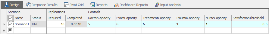
Figure 9.18: Controls for an experiment for Model 9-1.
In order to simulate a resource allocation problem, we need to assign costs for each unit of the various resources to be allocated. In Model 9-1, we are interested in the numbers of exam rooms, treatment rooms, trauma rooms, doctors and nurses. Table 9.2 gives the weekly resource costs that we’ll use. To offset the resource and staffing costs, we will also assign a waiting time cost of $250 for each hour of patient waiting time. This will allow us to explicitly model the competing objectives of minimizing the resource costs and maximizing the patient satisfaction (no one likes to wait after all).
| Resource | Weekly cost |
|---|---|
| Exam Room | $2,000 |
| Treatment Room | $2,500 |
| Trauma Room | $4,000 |
| Doctor | $12,000 |
| Nurse | $4,000 |
Since our model tabulates the total waiting time already, we can simply set our replication length to one week and can then calculate the total cost of a configuration as an output statistic. The expression that we use for the TotalCost output statistic is:
2000 x ExamCapacity + 2500 x TreatmentCapacity + 4000 x TraumaCapacity + 4000 x NurseCapacity + 12000 x DoctorCapacity + 250 x TotalWaitingTime.Value
Now we have two output statistics that we can use to evaluate system configurations — total cost and service level – total cost we want to be as low as possible and service level we want to meet a minimum value set by the stakeholders. Figure 9.19 shows a sample experiment (InitialExperiment) with four scenarios and the two output statistics defined as experiment Responses (TC for Total Cost and Satisfaction for the service level). In the model implementation, we divided the TotalCost value by 10,000 in the definition of the TC response so that it would be easier to compare the results visually in the experiment table (clearly, the division merely changes the measurement units and does not alter the comparative relationship between scenarios in any way). In the sample experiment, we ran the model for 7 days.
Finally, note that we just made up all of the costs in our model so that the model would be interesting. In the real world, these are often difficult values to determine/identify. In fact, one of the most important things to which to expose students in an educational environment is the difficulty in finding or collecting accurate model data.
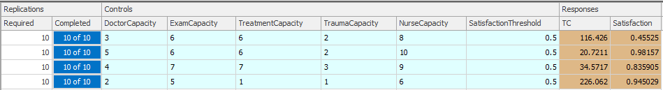
Figure 9.19: Initial experiment results for Model 9-1.
Since our total cost metric uses patient waiting time, we need to incorporate a warm-up period so that we can evaluate the system at steady state. When we use the Warm-up Period property in the Simio Experiment, model statistics are reset at the of the warm-up period. However, since we use a a model state (TotalWait) to accumulate the total patient waiting time, we need to manually reset this state at the end of the warm-up period (since, unlike the statistics elements, Simio has no way to know that this state needs to be reset). We can easily do this using an Assign step in the built-in OnRunWarmUpEnding process (see Figure 9.20). To access the process, click on the Select Process button from the Process ribbon.
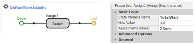
Figure 9.20: Resetting TotalWait at the end of the warm-up period.
Figure 9.21 shows the experiment after incorporation of the warm-up period. Here, the run length is 10 days and the warm-up period is 3 days.
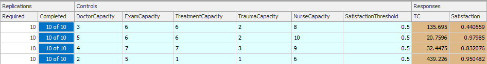
Figure 9.21: Experiment results for Model 9-1 with warm-up period.
9.1.1 Seeking Optimal Resource Levels in Model 9-1 With OptQuest
Hospital management would like to select just the right values for the five capacity levels (for each of Doctor, Exam, Treatment, Trauma, and Nurse) that will minimize Total Cost (TC), while at the same time providing an “adequate” service level, defined as resulting in a high proportion of Routine patients whose total waiting time is a half hour or less. Management feels that “adequate” service means that this proportion is at least 0.8; in other words, no more than 20% of Routine patients should have a total wait in excess of a half hour (of course this is all totally subjective and the “right” values for the threshold total waiting time and satisfaction percentage should be determined by stakeholders). Each of the five capacity levels must be an integer, and must be at least two (except that Trauma could be as low as one); management also wants to limit the capacities of Doctor to at most ten and Nurse to at most fifteen, and the capacities of Exam and Treatment to at most ten each, and Trauma to at most five.
Let’s think for a moment about what all this means. We’re trying to minimize total cost, an output response from the Simio model, so at first blush it might seem that the best thing to do from that standpoint alone would be to set each of the five capacity levels to the minimum allowed, which is two for each, except one for Trauma. However, remember that total cost includes a penalty of $250 for each hour of patient waiting time, which drives up total cost if we choose such rock-bottom capacity levels that, in turn, lengthen the queues (so maybe that’s not such a good idea after all, from the total-cost viewpoint). Likewise, we need to meet the service-level-satisfaction requirement, that it be at least 0.8, which may imply staffing some capacity levels above their bare-minimum values.
It helps our understanding of the situation to write all this out as a formal optimization problem, even though standard mathematical-programming methods (like linear programming, nonlinear programming, or integer programming) can’t even come close to actually solving it, since the objective function is an output Response from the simulation, so is stochastic (i.e., is subject to sampling error so we can’t even measure it exactly — more on this later). But, we can still at least express formally what we’d like to do:
\[\begin{eqnarray*} \min & TotalCost\\ \textrm{Subject to:}\\ & 2 \le DoctorCapacity \le 10\\ & 2 \le ExamCapacity \le 10\\ & 2 \le TreatmentCapacity \le 10\\ & 1 \le TraumaCapacity \le 5\\ & 2 \le NurseCapacity \le 15\\ & \textrm{All five of the above capacities are integers}\\ & Satisfaction \ge 0.8, \end{eqnarray*}\]
where the minimization is taken over DoctorCapacity, ExamCapacity, TreatmentCapacity, TraumaCapacity, and NurseCapacity jointly. The objective function that we’d like to minimize is TotalCost, and the lines after “Subject to” are constraints (the first six on input controls, and the last one on another, non-objective-function output). Note that the first five constraints, and the integrality constraint listed sixth, are on the input Controls to the simulation, so we know when we set up the Experiment whether we’re obeying all the range and integrality constraints on them. However, Satisfaction is another output Response (different from the total-cost objective) from the Simio model so we won’t know until after we run the simulation whether we’re obeying our requirement that it ends up being at least 0.8 (so this is sometimes called a requirement, rather than a constraint, since it’s on another output rather than on an input).
Well, it’s fine and useful to write all this out, but how are you going to go about actually solving the optimization-problem formulation stated above? You might first think of expanding the sample Experiment in Figure 9.19 for more Scenario rows to explore more (all, if possible) of the options in terms of the capacity-level controls, then sort on the TC (total-cost) response from smallest to largest, then go down that column until you hit the first “legal” scenario, i.e., the first scenario that satisfies the service-level Satisfaction requirement (the Satisfaction response is at least 0.8). Looking at the range and integrality constraints on the staffing Capacity levels, the number of possible (legal) scenarios is 9 x 9 x 9 x 5 x 14 = 51,030, a lot of Scenario rows for you to type into your Experiment (and to run). And, we need to replicate each scenario some number of times to get decent (sufficiently precise) estimates of TotalCost and Satisfaction. Some initial experimentation indicated that to get an estimate of TotalCost that’s reasonably precise (say, the half width of a 95% confidence interval on the expected value is less than 10% of the average) would require about 120 replications for some combinations of staffing capacities, each of duration ten simulated days — for each scenario. On a quad-core 3.0GHz laptop, each of these replications takes about 1.7 seconds, so to run this experiment (even if you could type in 51,030 Scenario rows in the Experiment Design) would take 51,030 \(\times\) 1.7 \(\times\) 120 seconds, which is some 120 days, or about four months. And, bear in mind that this is just a small made-up illustrative example — in practice you’ll typically encounter much larger problems for which this kind of exhaustive, complete-enumeration strategy is ridiculously unworkable in terms of run time.
So we need to be smarter than that, especially since nearly all of the four months’ of computation would be spent simulating scenarios that are either inferior in terms of (high) TotalCost, or unacceptable (i.e., infeasible) due to their resulting in a Satisfaction proportion less than the required 0.8. If you think of our optimization formulation above in terms of just the five input capacity-level controls, you’re searching through the integer-lattice points in a five-dimensional box, and maybe if you start somewhere in there, and then simulate at “nearby” points in the box, you could get an idea of which way to move, both to decrease TotalCost, and to stay feasible on the Satisfaction requirement. It turns out that there’s been a lot of research done on such heuristic-search methods to try to find optima, mostly in the world of optimizing difficult deterministic functions, rather than trying to find an optimal simulation-model configuration, and software packages for this have been developed. One of them, OptQuest (from OptTek Systems, Inc., www.opttek.com), has been adapted to work with Simio and other simulation-modeling packages, to search for a near-optimal feasible solution to problems like our hospital-capacities problem. There’s a large literature on all this, and a good place to start is the open-access Winter Simulation Conference tutorial (Glover, Kelly, and Laguna 1999); for more, see the handbook (Glover and Kochenberger 2003).
Using results and recommendations from this body of research, OptQuest internally decides which way to move from a particular point (the user must provide a starting point, i.e. five initial capacities in our problem) in the five-dimensional box to try to improve the objective-function value (reduce total cost in our example), while obeying the constraints on the input parameters (the ranges on our five capacities) and also obeying any constraints/requirements on other outputs (checking that Satisfaction \(\ge 0.8\) for us). Though our example doesn’t have it, OptQuest also allows you to specify constraints on linear combinations of the five capacities, e.g., \(5 \le DoctorCapacity + NurseCapacity \le 20,\) for which we’d need to specify two constraints with a single inequality in each. OptQuest uses a combination of heuristic search techniques (including methods known as scatter search, tabu search, and neural networks) to find a much more efficient route through the 5D box toward an optimal point — or, at least a good point that’s almost certainly better than we could ever find by just trying scenarios haphazardly on our own, as these methods cannot absolutely guarantee that they’ll find a provably optimal solution. As stated in (Glover, Kelly, and Laguna 1999),
… a long standing goal in both the optimization and simulation communities has been to create a way to guide a series of simulations to produce high quality solutions The optimization procedure uses the outputs from the simulation model which evaluate the outcomes of the inputs that were fed into the model. On the basis of this evaluation, and on the basis of the past evaluations which are integrated and analyzed with the present simulation outputs, the optimization procedure decides upon a new set of input values … The optimization procedure is designed to carry out a special “non-monotonic search,” where the successively generated inputs produce varying evaluations, not all of them improving, but which over time provide a highly efficient trajectory to the best solutions. The process continues until an appropriate termination criterion is satisfied (usually given by the user’s preference for the amount of time to be devoted to the search).
For a deeper discussion of scatter search, tabu search, neural networks, and how OptQuest uses them, see (Glover, Kelly, and Laguna 1999) and (Glover and Kochenberger 2003).
The way OptQuest works with Simio is that you describe the optimization formulation in a Simio Experiment, including identifying what you want to minimize or maximize (we want to minimize total cost), the input constraints (the capacity ranges for us, and that they must be integers), and any other requirements on other, non-objective-function outputs (the Satisfaction-proportion lower bound of 0.8). Then, you turn over execution of your Experiment and model to OptQuest, which goes to work and decides which scenarios to run, and in what order, to get you to a good (even if not provably optimal) solution in a lot less than four months’ worth of nonstop computing. One of the time-saving strategies that OptQuest uses is to stop replicating on a particular scenario if it appears pretty certain that this scenario is inferior to one that it’s already simulated — there’s no need to get a high-precision estimate of a loser.
Here’s how you set things up for OptQuest in a Simio experiment. First, we’ll create a new Simio Experiment (choose the New Experiment button from the Project Home ribbon) so that we can experiment both with and without OptQuest. We named the experiment OptQuest1. Next, we need to tell Simio to attach the OptQuest for Simio add-in. An experimentation add-in is an extension to Simio (written by the user or someone else — see the Simio documentation for details about creating add-ins) that adds additional design-time or run-time capability to experiments. Such an add-in can be used for setting up new scenarios (possibly from external data), running scenarios, or interpreting scenario results. Combining all three technologies can provide powerful tools, as illustrated by the OptQuest for Simio add-in. To attach the add-in, select the Add-In button on the experiment Design ribbon and choose the OptQuest for Simio option from the list (see Figure 9.22).
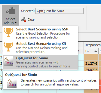
Figure 9.22: Selecting the OptQuest Add-in.
Note that when you select OptQuest, you may get a warning similar to “Setting an add-in on an experiment cannot be undone. If you set the add-in, the current undo history will be cleared. Do you want to continue?” If you need to keep the undo history (and we can’t think of a reason why this would ever be the case, but you never know!), you should answer No, make a copy of the model, and open the copy to set up for OptQuest. Otherwise, just answer Yes and Simio will load the add-in (and, of course, clear the undo history). Once you’ve the added OptQuest add-in, your experiment will have some additional properties that control how OptQuest works (see Figure 9.23).
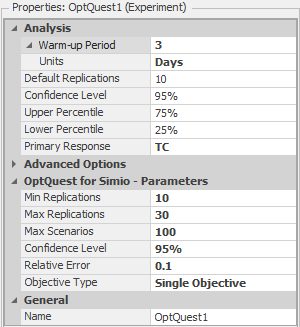
Figure 9.23: Experiment properties for OptQuest1 after attaching the OptQuest Add-in.
The OptQuest-related properties are:
- Min Replications: The minimum number of replications Simio should run for each OptQuest-defined scenario.
- Max Replications: The maximum number of replications Simio should run for each OptQuest-defined scenario.
- Max Scenarios: The maximum number of scenarios Simio should run. Basically, OptQuest will systematically search for different values of the decision variables — the number of Doctors, Exam Rooms, Treatment Rooms, Trauma Rooms, and Nurses, in our case — looking for good values of the objective (small values of Total Cost, in our case), and also meeting the Satisfaction-proportion requirement that it be at least 0.8. This property will limit how many scenarios OptQuest will test. Note that OptQuest will not always need this many scenarios, but the limit will provide a forced stopping point, which can be useful for problems with very large solution spaces. But, you should realize that if you specify this property to be too small (though it’s not clear how you’d know ahead of time what “too small” might mean), you could be limiting the quality of the solution that OptQuest will be able to find.
- Confidence: The confidence level you want OptQuest to use when making statistical comparisons between two scenarios’ response values.
- Error Percent: Percentage of the sample average below which the half-width of the confidence interval must be. For example, if the sample average is 50 and you set the Error Percent to 0.1 (which says that you want the confidence-interval half-width to be at most 10% of the average, so roughly speaking 10% error), the confidence-interval will be at least as precise as 50 \(\pm 5\) (\(5=0.1 \times 50\)). After running the default number of replications, OptQuest will determine if this condition has been satisfied. If not, Simio will run additional replications in an attempt to reduce the variability to achieve this goal (until it reaches the number of replications specified by the Max Replications property value).
Attaching the OptQuest add-in also adds properties to the experiment controls. With the OptQuest add-in, we can specify the optimization constraints using either the experiment controls or Constraints — we’ll use the experiment controls for the current model since each of the constraints involves limiting the values of a single control (a Referenced Property in the model). If we had had linear combination-type constraints such as the one above that limits the total number of doctors and nurses, we would have used an experiment Constraint.
Figure 9.24 shows the properties for the Doctor Capacity control after attaching the OptQuest add-in (note that prior to attaching the add-in, there were no user-editable properties for experiment controls).
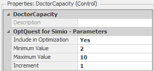
Figure 9.24: Properties for the Doctor Capacity control after attaching OptQuest.
The “new” control properties tell OptQuest whether it should manipulate the control to search the feasible region (Include in Optimization), the “legal” values for the control (between and including the Minimum Value and Maximum Value property values), and the increment (Increment property value) to use when searching the feasible region from one point to the next. The control properties shown in Figure 9.24 specify the constraint on the Doctor Capacity from the optimization model above (i.e., integers between 2 and 10, inclusive). The corresponding properties for the Exam Capacity, Treatment Capacity, Trauma Capacity, and Nurse Capacity controls are set similarly. Since we’re not using the Satisfaction Threshold control in our optimization (recall that we used a referenced property to specify the threshold), we set the Include in Optimization property to No. For a control that’s not used in the optimization, Simio will use the default value (0.5 in this case) for the property in all scenarios.
The only remaining “constraint” from our optimization above is the requirement on the Satisfaction level (recall that we called this a requirement rather than a constraint since Satisfaction is an output rather than an input). Figure 9.25 shows the properties for the Satisfaction response (note that, with the exception of setting the Lower Bound property to 0.8, this response is the same as the corresponding Satisfaction response in the previous experiment).

Figure 9.25: Properties for the Satisfaction Response.
The final step for setting up OptQuest is to define the objective function — i.e., tell OptQuest the criterion for optimization. Since we’d like to minimize the total cost, we’ll define the TC response (as we did before) and specify the Objective property as Minimize (see Figure 9.26).
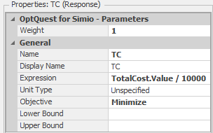
Figure 9.26: Properties for the TC response.
As mentioned earlier, we divided the TotalCost value by 10,000 in the definition of the TC response so that it would be easier to compare the results visually in the experiment table. Finally, we’ll set the experiment property Primary Response to TC to tell OptQuest that the TC response (minimizing TC in this case) is the objective of the optimization.
Now you can click the Run button and sit back and watch OptQuest perform the experiment. Figure 9.27 shows the “top” several scenarios from the OptQuest run (we sorted in increasing order of Total Cost, so the top scenario has the minimum total cost of the scenarios tested). The figure also shows some scenarios from further down in the sorted list (starting with Scenario 071). Note: Depending on the specific version of Simio that you are running, you may see different scenarios in the list, but specific configurations should have similar responses values.These differences can be caused by differences in the number of processors/cores, processor speed, and computational load at the time of the run.
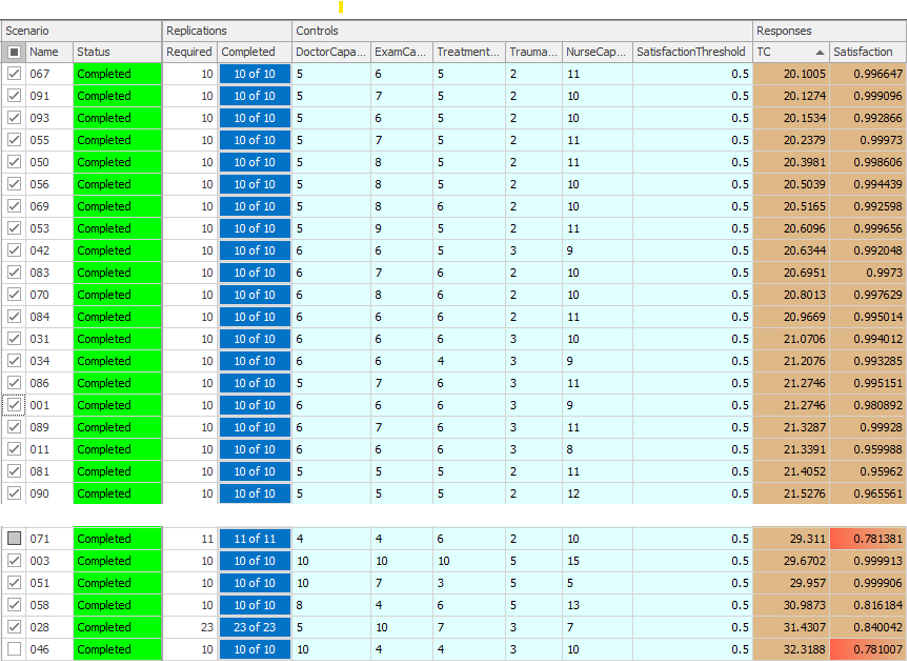
Figure 9.27: Results for the initial OptQuest run (two sections from the experiment table).
The top scenario in the list is scenario \(067\), which has 5 Doctors, 6 Exam Rooms, 5 Treatment Rooms, 2 Trauma Room and 11 Nurses, a Total Cost of \(20.1005\) (in ten-thousands) and a Satisfaction of \(0.997\). Note that all of the Satisfaction values are quite high – you have to go down the list of scenarios to scenario \(071\) before you find an infeasible solution (one where the 80% satisfaction requirement is not met — note that the Satisfaction value has red background and scenario is unchecked, indicating infeasibility). Naturally, the next question should be “Is this really the truly optimal solution?” Unfortunately, the answer is that we’re not sure. As mentioned earlier, OptQuest uses a combination of heuristic-search procedures, so there is no way (in general) to tell for sure whether the solution that it finds is truly optimal. Remember that we identified \(51,030\) possible configurations for our system and that we limited OptQuest to testing 100 of these. Such is the nature of heuristic solutions to combinatorial optimization problems. We’re pretty confident that we have good solutions, but we just don’t know with absolute certainty that we have “the” optimum, upon which no improvement is possible.
While we can’t say with any certainty that OptQuest finds the best solution, it’s quite likely that OptQuest can do better than you (or we) could do by just arbitrarily searching through the feasible region (especially after you’ve reached your 37th scenario and are tired of looking at the computer). Where OptQuest can be really useful is in cases where you can limit the size of the feasible region. For example, we constrained the number of Trauma Rooms in our problem to be between 1 and 5, but the expected arrival rate of Urgent patients (the only patients that require the Trauma room) is quite low (about 0.6 per hour). As such, it is extremely unlikely that we would ever need more than 1 or 2 trauma rooms. If we change the upper limit on the Trauma Room control from 5 to 2, we reduce the size of the feasible region from 51,030 to 20,412 and can likely improve the performance of OptQuest for a smaller number of allowed scenarios. There are clearly other similar adjustments we could make to the experiment to reduce the solution space. This highlights the importance of your being involved in the process — OptQuest doesn’t understand anything about the specific model that it’s running or the characteristics of the real system you’re modeling, but you should, and making use of your knowledge can substantially reduce the computational burden or improve the final “solution” on which you settle. Now we’ll turn our attention to evaluating the scenarios that OptQuest has identified, hopefully to identify the “best” scenario.
9.1.2 Ranking and Selection of Alternate Scenarios in Model 9-1 With Subset Selection and KN
Since the response values shown in Figure 9.27 are sample means across ten replications of each scenario, they are subject to sampling error. As such, we’re not sure that this ordering, based on these sample means from the OptQuest experiment, identifies the true optimum of our problem (i.e., the best configuration of our resources in terms of lowest total cost). Figure 9.28 shows the SMORE plots for the top five scenarios from our OptQuest run. While the sample mean of total cost (TC) for scenario 051 is clearly the lowest compared to the sample means of the other scenarios, when we take the confidence intervals into consideration through a visual comparison of the SMORE plots, things are no longer so clear. In fact, in looking a Figure 9.28 it’s difficult to tell if there are statistically significant differences between the five sample means (while visual inspection of SMORE plots cannot accurately identify true statistically significant differences, it can still guide further analysis). Our uncertainty here stems from sampling uncertainty, and this is exactly is where Subset Selection Analysis comes into play, as discussed earlier in Section 5.5 in a smaller example than the one we consider here.
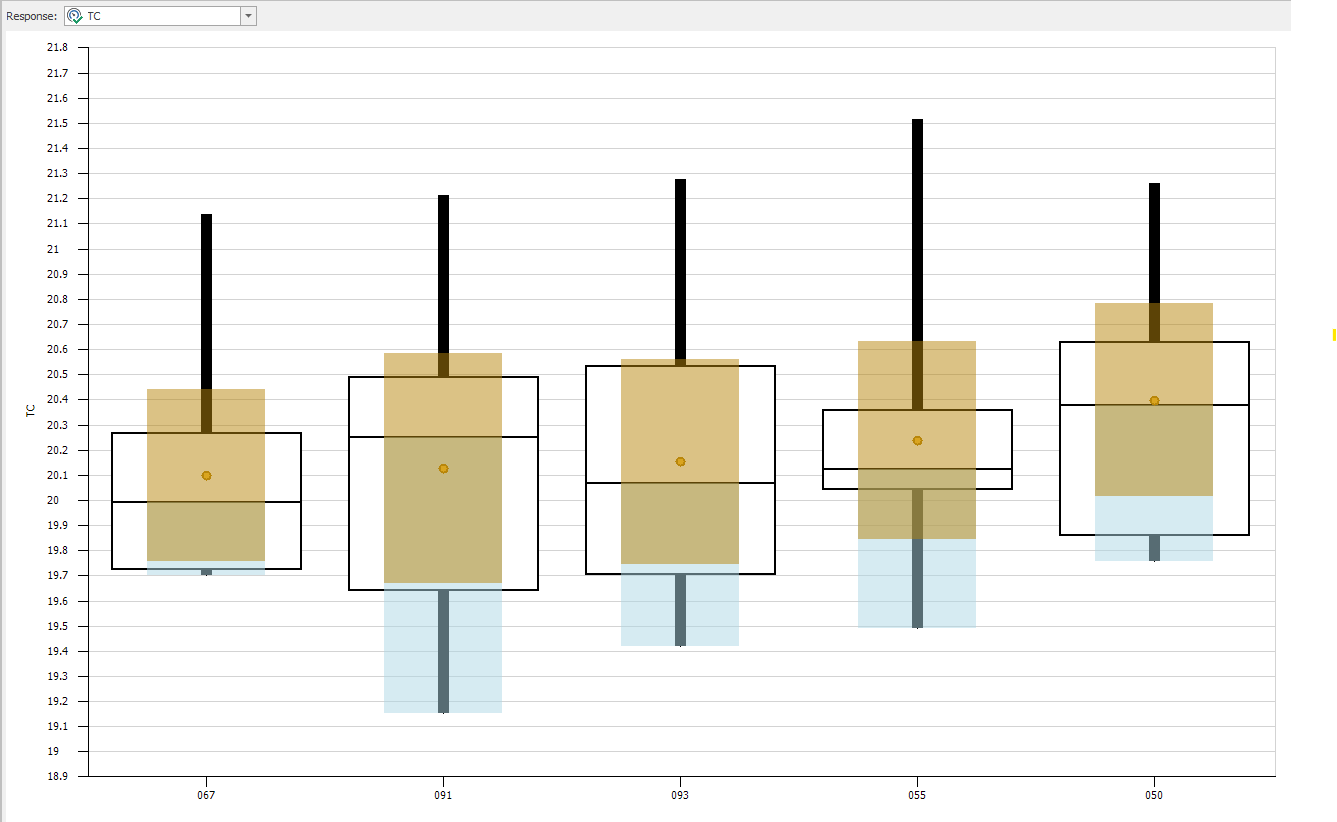
Figure 9.28: SMORE plots for the top five scenarios from the OptQuest run of Model 9-1.
Figure 9.29 shows the results from a second OptQuest run where we changed the upper limit on the Trauma Room to 2 and the Max Scenarios to 25 and then ran the Subset Selection Analysis function (by clicking its icon on the Design ribbon). This function considers the replication results for all scenarios and divides the scenarios into two groups: the “possible best” group, consisting of the scenarios with responses shaded darker brown and whose sample means are statistically indistinguishable from the best sample mean; and the “rejects” group, consisting of the scenarios whose responses are shaded lighter brown. Based on this initial experimentation of ten replications per scenario, the scenarios in the “possible best” group warrant further study, while those in the “rejects” group are statistically “worse” and do not need further consideration (with respect to the given response). You should not interpret the scenarios in the “possible best” group as having in some sense “proven” themselves as “good” — it’s just that they have not (yet) been rejected. This asymmetry is akin to classical hypothesis testing where failure to reject the null hypothesis in no way connotes any sort of “proof” of its truth — we just don’t have the evidence to reject it; on the other hand, rejecting the null hypothesis implies fairly convincing evidence that it’s false. Note that if no scenarios in your experiment are identified as “rejects,” it is likely that your experiment does not include enough replications for the Subset Selection procedure to identify statistically different groups. In this case, running additional replications should fix this problem (unless there actually are no differences between the scenarios).
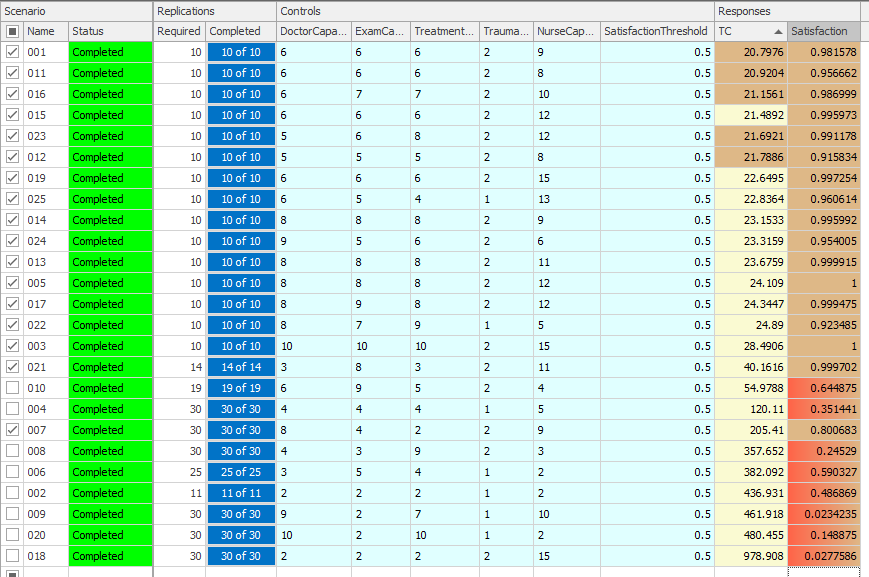
Figure 9.29: Results for the second OptQuest run after running Subset Selection Analysis.
In our example, the dark-brown “possible best” group includes five feasible scenarios (see Figure 9.29). Clearly, the question at this point is “What now?” We have a choice between two basic options: Declare that we have five “good” configurations, or do additional experimentation. Assuming that we want to continue to try to find the single best configuration (or at least a smaller number of possible-best scenarios), we could run additional replications of just the five scenarios in the current “possible best” group and re-run the Subset Selection Analysis to see if we could identify a smaller “possible best” group (or, with some luck, the single “best” scenario). We unselected the scenarios in the current “rejects” group from the experiment and ran the remaining five scenarios for an additional 40 replications each (for a total of 50 replications each), and the resulting new “possible best” group (not shown) contained only four feasible scenarios; note that you must “Clear” the OptQuest add-in prior to running the additional scenarios, by clicking on the Clear icon in the Add-ins section of the Ribbon. As before, we can either declare that we have four “good” configurations, or do additional experimentation. If we want to continue searching for the single “best” configuration, we could repeat the previous process — delete the scenarios in the most recent “rejects” group and run additional replications with the remaining scenarios. Instead, we will use another Simio Add-in to assist in the process.
The add-in Select Best Scenario using KN, based on (Kim and Nelson 2001) by Kim and Nelson, is designed to identify the “best” scenario from a given set of scenarios, as mentioned in Section 5.5. The add-in continues to run additional replications of the candidate scenarios, one replication at a time, until it either determines the “best” or exhausts the user-specified maximum number of scenarios. To run the KN add-in, choose Select Best Scenario using KN using the Select Add-In icon in the Design ribbon, just as we did when we used OptQuest earlier (see Figure 9.22). This will expose some additional experiment properties related to the add-in (see Figure 9.30).
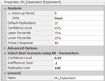
Figure 9.30: Experiment properties after including the Select Best Scenario using KN add-in.
In addition to the Confidence Level property (that specifies the level to use for confidence intervals), you also specify the Indifference Zone and Replication Limit. The Indifference Zone is the smallest “important” difference that should be detected. For example, 21.65 and 21.68 are numerically different, but the difference of 0.03 may be unimportant for the particular problem (clearly the appropriate choice of an indifference-zone value depends on what the response is measuring, and on the context of the study). An indifference zone of 0.10 would cause the add-in not to differentiate between these values during the experimentation. While it might be tempting to declare a very small indifference zone, in effect saying that you’re a demanding perfectionist and care about even tiny suboptimalities, you should be aware that you’ll pay a potentially heavy price for this in terms of large numbers of replications, and thus very long computing times, required to achieve such high resolution (the amount of computing can grow superlinearly as the indifference zone is squeezed down tighter). The Replication Limit tells the add-in the maximum number of replications to run before “giving up” on finding the best scenario (and declaring the remaining scenarios “not statistically different”).
Figure 9.31 shows the experiment after running the add-in, which identified scenarios 001, 016, and 011 as the “best” configurations, per the checked box in the leftmost column, after running these scenarios for 100 replications (the KN procedure, not the user, determined these numbers of replications). If the add-in terminates with multiple scenarios checked, it cannot differentiate between the checked scenarios based on the maximum number of replications (which we specified to be 100 in this example) and the Indifference Zone. Note that the first scenario (001) is the same scenario that had minimum average total cost after our second OptQuest run (Figure 9.29), but the the total cost for Scenario 001 is higher (\(21.045\) here vs.~\(20.798\) earlier) after running the additional replications. A quick glance at the SMORE plots (not shown) shows a fairly small confidence interval around our sample mean, indicating that the initial results from our ten replications in the OptQuest experiment very likely resulted in a low value for their sample mean. This illustrates the need to pay close attention to the confidence intervals and run more replications where necessary before using the experiment results to make decisions.

Figure 9.31: Experiment results after running the Select Best Scenario using KN add-in.
A full description and justification of the KN selection procedure is beyond our scope, but briefly, it works as follows. An initial number of replications is made of all scenarios still in contention to be the best (at the beginning, all scenarios are “still” in contention), and the sample variances of the differences between the sample means of all possible pairs of scenarios is calculated. Based on these sample variances of differences between sample means, more replications are run of all surviving scenarios, one at a time, until there is adequate confidence that one particular scenario is the best, or at least within the indifference zone of the best; along the way the procedure eliminates scenarios that appear no longer to be candidates for the best, and no further replications of them are run, thus reducing the size of the set of scenarios still in contention (as a way to improve computational efficiency by not wasting further computing time on scenarios that appear to be inferior). If the user-specified limit on the number of replications (100 in our example) is reached before a decision on the best can be made, then all surviving scenarios still in contention are considered as possibly the best. Note the fundamental difference in approach between this KN select-the-best method vs. subset selection — with subset selection we made a fixed number of replications then subset selection did its best to divide the scenarios into “possible best” vs. “rejects” on the basis of this fixed “sample size,” whereas the KN select-the-best took as fixed the user’s desire to identify the single best scenario and called for as many replications as necessary of the scenarios to do so. Compared to earlier such methods, KN has at least a couple of important advantages. First, it is fully sequential, i.e. takes additional replications just one at a time, in contrast to two-stage sampling where multiple replications are made in a single second stage after the initial number of replications, thereby possibly “overshooting” the number of replications really required (which is unfortunate for large complex models where making a single replication could take many minutes or even hours). Second, it is valid whether or not common random numbers across scenarios are being synchronized to try to reduce the underlying true variances in the differences between the sample means. For full detail on KN see the original paper (Kim and Nelson 2001).
Another closely related approach is the add-in Select Best Scenario using GSP. The GSP add-in is a scenario selection algorithm with good performance for large scale models. This add-in is similar to the KN add-in described above, but may provide improved performance when doing larger scale models that require evaluation of many scenarios in a parallel processing environment. This add-in was created by Sijia Ma as part of his PhD work at Cornell University. For more information on both scenario selection algorithms search “Select Best Scenario” in the Simio Help.
To summarize, we started by using the OptQuest add-in to identify potentially promising scenarios (configurations with specific values for the referenced properties) based on our optimization formulation. After running OptQuest, we used the Subset Selection Analysis function to partition the set of scenarios into the “possible best” and “rejects” groups. We then did further experimentation with the scenarios in the “possible best” subset. We first ran additional replications to reduce the size of this subset, and finally used the Select Best Scenario using KN add-in to identify the “best” configuration. Since we are using heuristic optimization and generally will not be able to evaluate all configurations in the design space, we will generally not be able to guarantee that our process has found the best (or even very good) configurations, but experience has shown that the process usually works quite well, and once again, much better than we could expect to do on our own with just some essentially arbitrarily-defined scenarios and haphazard experimentation.
9.2 Model 9-2: Pizza Take-out Model
In Model 9-2 we will also consider a related resource allocation problem. The environment that we are modeling here is a take-out pizza restaurant that takes phone-in orders and makes the pizzas for pickup by the customer. Customer calls arrive at the rate of 12 per hour and you can assume that the call interarrival times are exponentially distributed with mean 5 minutes. The pizza shop currently has four phone lines and customers that call when there are already 4 customers on the phone will receive a busy signal. Customer orders consist of either 1 (50%), 2 (30%), 3 (15%), or 4 (5%) pizzas and you can assume that the times for an employee to take a customer call are uniformly distributed between 1.5 and 2.5 minutes. When an employee takes an order, the shop’s computer system prints a “customer ticket” that is placed near the cash register to wait for the pizzas comprising the order. In our simplified system, individual pizzas are made, cooked, and boxed for the customer. Employees do the making and boxing tasks and a semi-automated oven cooks the pizzas.
The make station has room for employees to work on three pizzas at the same time although each employee can only work on one pizza at a time. The times to make a pizza are triangularly distributed with parameters 2, 3, and 4 minutes. When an employee finishes making a pizza, the pizza is placed in the oven for cooking. The cooking times are triangularly distributed with parameters 6, 8 and 10 minutes. The oven has room for eight pizzas to be cooking simultaneously. When a pizza is finished cooking, the pizza is automatically moved out of the oven into a queue where it awaits boxing (this is the “semi-automated” part of the oven). The boxing station has room for up to three employees to work on pizzas at the same time. As with the make process, each employee can only be working on one pizza at a time. The boxing times are triangularly distributed with parameters 0.5, 0.8, and 1 minutes (the employee also cuts the pizza before boxing it). Once all of the pizzas for an order are ready, the order is considered to be complete. Note that we could also model the customer pick-up process or model a home delivery process, but we will leave this to the interested reader.
The pizza shop currently uses a pooled employee strategy for the order-taking, pizza making, and pizza boxing processes. This means that all of the employees are cross-trained and can perform any of the tasks. For the make and box operations, employees need to be physically located at the respective stations to perform the task. The shop has cordless phones and hand-held computers, so employees can take orders from anywhere in the shop (i.e., there is no need for a physical order-taking station).
Figure 9.32 shows the Facility view of the completed version of Model 9-2. Note that we have defined Customer and Pizza entity types and have labeled the entities using Floor Labels. The Floor Labels allow us to display model and entity states on the labels. Floor Labels that are attached to entities will travel with the entities.
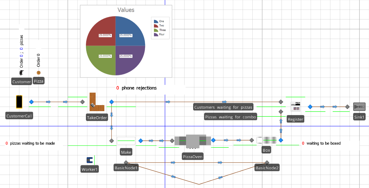
Figure 9.32: Facility view for Model 9-2.
To create a Floor label for an entity, simply select the entity, in the Facility view, click on the Floor Label icon on the Attached Animation ribbon (since the label is attached to the entity), and place the label by clicking, dragging, and clicking on the Facility view where you would like the label. This will create a label with default text including instructions for formatting the label. Clicking on the Edit icon in the Appearance ribbon will bring up an edit dialog box (see Figure 9.33) for the Pizza entity Floor label. Note the use of the OrderNumber entity state set off by braces. To rotate the label, select the label, click and hold the Ctrl key and click on one of the corners (the green circles). The circle will turn red and you can rotate the label as long as you hold the Ctrl key. Note that this general process can be used to rotate any object in the Facility View.
As the model executes, this place-holder will be replaced with the entity state value (the order number for the specific pizza). The model also has a Source object (CustomerCall) and Server objects for the order taking (TakeOrder), making (Make), and boxing (Box) processes and the oven (PizzaOven). The model includes a Combiner object (Register) for matching the Customer objects with the Pizza objects representing the pizzas in the order and a single Sink object where entities depart. Finally, in addition to the Connector objects that facilitate the Customer and Pizza entity flow, we add a Path loop between two Node objects (BasicNode1 and BasicNode2) that will facilitate employee movement between the make station and the box station. If you are following along, you should now place all of the objects in your model so that the Facility view looks approximately like that in Figure 9.32.
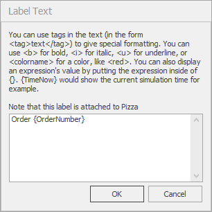
Figure 9.33: Edit dialog box for the Pizza entity Floor Label.
The CustomerCall Source object creates the customer calls based on the specific customer arrival process described above (the Interarrival Time property is set to Random.Exponential(5) minutes). Note that the model includes Customer and Pizza entity types so that Entity Type property for the Source object is set to Customer. Customer calls are then sent to the TakeOrder Server object for potential processing. Recall that if there are already four callers in the system, the potential customer receives a busy signal and hangs up. We will model this capacity limitation using an add-on process. Since we need to make a yes/no decision before processing the customer order, we will use an add-on process associated with the Input node for the TakeOrder object and will reject the call if the call system is at capacity. We will use the Entered trigger so that the process is executed when an entity enters the node. Figure 9.34 shows the Input_TakeOrder_Entered add-on process.
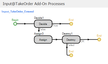
Figure 9.34: Add-on process for the input node of the TakeOrder object.
The Decide step implements a condition-based decision to determine whether there is a phone line available. We model the number of phone lines using the TakeOrder object capacity and the associated Input Buffer capacity. Figure 9.35 shows the properties for the TakeOrder object. Note that we have set the Initial Capacity property to 1 and the Input Buffer property to a referenced property named NumLines. Our Decide step therefore uses the following expression to determine whether or not to let a call in: TakeOrder.InputBuffer.Capacity.Remaining > 0. If the condition is true, the call is allowed into the TakeOrder object. Otherwise, we increment the PhoneRejections user-defined model state to keep track of the number of rejected calls and destroy the entity. So based on the TakeOrder object properties and the Input_TakeOrder_Entered add-on process a maximum of one employee can be taking an order at any time and the number of customers waiting “on hold” is determined by the value of the NumLines referenced property. Note that our use of a referenced property to specify the input buffer capacity will simplify experimenting with different numbers of phone lines (as we will see soon). For the base configuration described above, we would set the referenced property value to 3 to limit the number of customers on the phone to a total of 4.
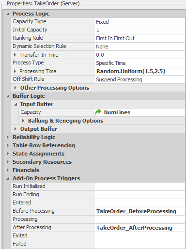
Figure 9.35: Properties for the TakeOrder object.
Once a customer enters the system, an employee will take the call and process the order. We use a Worker object (Worker1) to model our pooled employees. Figure 9.36 shows the properties for the Worker1 object. Recall from Chapter 8 that the Worker object will allow us to model workers that move and have an associated physical location within the model. Below, we will define locations for the make and box stations and will track the location of each of the employees. As such, we set the Initial Desired Speed property to 1 meter per second, the Initial Network to the WorkerNetwork, and the Initial Node (Home) to BasicNode2 (we defined the WorkerNetwork using BasicNode2 below the box station and BasicNode1 below the make station along with the Path objects comprising the loop that the Worker objects use to move between the two stations). Note that we also used a referenced property (NumWorkers) for the Initial Number In System property so that we can easily manipulate the number of workers during experimentation. As we did in Model 9-1, we will use a Seize step to seize a Worker1 resource in the Processing add-on process for the TakeOrder object (see Figure 9.35). If a Worker1 resource is not available, the entity will wait at the Seize step. Since the employee can take the order from anywhere in the shop, we have no requirement to request the Worker1 object to actually move anywhere, we simply need the resource to be allocated to the order taking task. In the real pizza shop, this would be equivalent to the employee answering the cordless phone and entering the order via the hand-held computer from wherever she/he is in the shop. This will not be the case when we get to the Make and Box stations below.
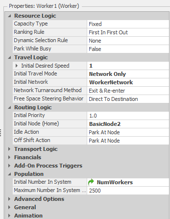
Figure 9.36: Properties for the Worker1 object.
Once the Worker1 resource is allocated, the entity is delayed for the processing time associated with actually taking the customer order. At this point, we need to create the associated Pizza entities and send them to the make station and send the Customer entity to wait for the completed Pizza entities to complete the order. This is done in the TakeOrder_AfterProcessing add-on process (see Figure 9.37).
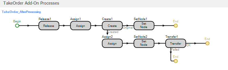
Figure 9.37: Processed add-on process for the TakeOrder object.
The first step in the process releases the Worker1 resource (since the call has been processed by the time the process executes). The first Assign step makes the following state assignments:
HightestOrderNumber=HighestOrderNumber+1— Increment the model state HighestOrderNumber to reflect the arrival of the current orderModelEntity.OrderNumber=HighestOrderNumber— Assigns the current order number to the Customer entityModelEntity.NumberOrdered=Random.Discrete(1,.5,2,.8,3,.95,4,1)— Determine the number of pizzas in this order and store the value in the entity state NumberOrderedNumberOrdered[ModelEntity.NumberOrdered]=NumberOrdered[ModelEntity.NumberOrdered]+1— This assignment increments a model state that tracks the number of orders at each size (number of pizzas in the order). Figure 9.38 shows the properties for theNumberOrderedmodel state. Note that it is a vector of size 4 – one state for each of the four potential order sizes. At any point in simulation time, the values will be the numbers of orders taken at each order size. Figure 9.39 shows the Status Pie chart along with the properties and repeat group used for the chart.
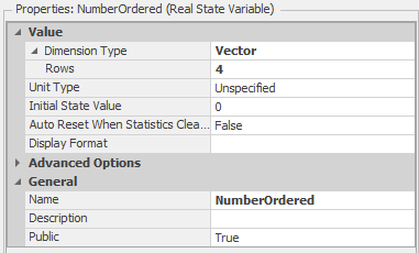
Figure 9.38: Properties for the NumberOrdered model state.

Figure 9.39: Properties for the NumberOrdered model state.
The Create step creates the Pizza entity objects using the NumberOrdered state to determine how many entities to create (see
Figure 9.40 for the Create step properties). Leaving the Create step, the original entity will move to the SetNode step and the newly created Pizza objects will move to the Assign step. The Set Node step assigns the destination Node Name property to ParentInput@Register, so that when the entity object leaves the TakeOrder object, it will be transferred to the Register object to wait for the Pizza entity objects that belong to the order (the Customer object represents the “customer ticket” described above). The Assign step assigns the ModelEntity.OrderNumber state the value HighestOrderNumber. Recall that the Customer object entity state OrderNumber was also assigned this value (see above). So the OrderNumber state can be used to match-up the Customer object with the Pizza objects representing pizzas in the customer order. The SetNode step for the newly created Pizza entity objects sets the destination Node Name property to Input@Make so that the objects will be transferred to the Make object. Finally, we have to tell Simio where to put the newly created objects (the Create step simply creates the objects in free space). The Transfer step will immediately transfer the object to the node specified in the Node Name property (Output@TakeOrder, in this case). So at this point, the Customer object will be sent to the register to wait for Pizza objects, the Pizza objects will be sent to the make station and all of the objects associated with the customer order can be identified and matched using the OrderNumber respective entity states.
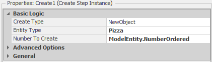
Figure 9.40: Properties for the Create step.
The Register Combiner object matches Customer objects representing customer orders with Pizza objects representing the pizzas that comprise the customer order. Figure 9.41 shows the properties for the Combiner object. The Batch Quantity property tells the Combiner object how many “members” should be matched to the “parent.” In our case, the parent is the Customer object and the members are the corresponding Pizza objects. As such, the ModelEntity.NumberOrdered entity state specifies how many pizzas belong to the order (recall that we used this same entity state to specify the number of Pizza objects to create above). The Member Match Expression and Parent Match Expression properties indicate the expressions associated with the member and parent objects to match the objects.
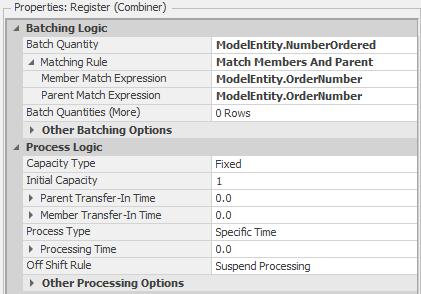
Figure 9.41: Properties for the Register Combiner object.
Figure 9.42 shows the Combiner object with a Customer object with label “Order 3; 1 pizzas” waiting in the parent queue and one Pizza objects with label Order 3 waiting in the member queue. Note how the Floor Labels help us identify the situation – 1 pizzas in in customer order 3, with the pizza boxed and waiting. When the final Pizza object arrives to the Combiner object, it will be combined with the other Pizza objects and the Customer object and the order will be complete. When this happens, the Customer object will leave the Combiner object and be transferred to the Sink object.
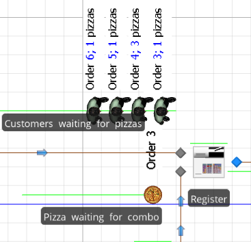
Figure 9.42: Combiner object with one parent and two member objects in queue.
The Make Server object models the pizza making station. Since the make station has room for three employees to be making pizzas simultaneously, we set the Initial Capacity property to 3. We also set the Processing Time property to Random.Triangular(2,3,4) minutes. Since the make process also requires an employee, we will use the BeforeProcessing add-on process to seize the Worker object and the AfterProcessing add-on process to release the worker as we have done previously with the TakeOrder object. The difference here is that the make process requires that the employee be physically present at the make station in order to make the pizza. As such, we need to request that the Worker object travel to BasicNode2 (the node in the WorkerNetwork designated for the make station). Luckily we can make this request directly when we seize the Worker object. Figure 9.43 shows the Seizes property editor associated with the Seize step in the Make_Processing add-on process. Here, in addition to specifying the Object Name property (Worker1), we also set the Request Visit property to ToNode and the Node Name property to BasicNode1 indicating that when we seize the object, the object should be sent to the BasicNode1 node. When the add-on process executes, the token will remain in the Seize step until the Worker object arrives at BasicNode. Finally, we set the Box Server object up similarly (except we set the Processing Time property to Random.Triangular(0.5,0.8,1) and specify that the Worker object should visit BasicNode2).
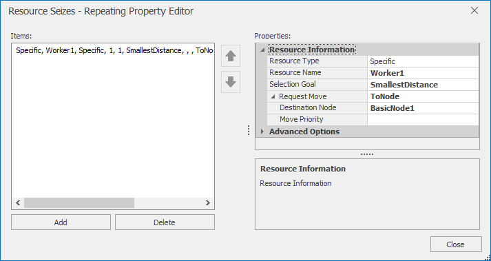
Figure 9.43: Seizes property editor for the Seize step in the Make Processing add-on process.
So our model is now complete — if a phone line is available when a customer call arrives, the first available employee takes the call and records the order. The corresponding Customer Order entity then creates the Pizza entities associated with the orders. The Customer Order entity is then sent to wait for the Pizza orders that comprise the order and the Pizza entities are sent for processing at the Make, Oven, and Box stations. Once all Pizza entities complete processing at the Box station, the Customer Order and Pizza entities for an order are combined and the order is complete. To support our experimentation, we used referenced properties to specify the number of phone lines (NumLines) and number of employees (NumWorkers).
9.2.1 Experimentation With Model 9-2
Figure 9.44 shows a simple 15-scenario experiment that we set up and ran for Model 9-2 (the run length was 1000 hours and there was no warmup – see Problem 3 at the end of the chapter to explore these choices). The number of phone lines (NumLines) and number of workers (NumWorkers) are the controls for the experiment. We have also defined three responses:
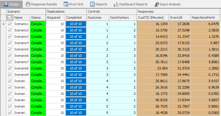
Figure 9.44: Simple experiment results for Model 9-2.
- CustTIS - the time that customer orders spend in the system. Defined as
Customer.Population.TimeInSystem.Average(make sure to set the Unit Type to Time and the Display Units to Minutes so that the response values will be shown in minutes); - Oven Util - the oven’s scheduled utilization. Defined as
PizzaOven.Capacity.ScheduledUtilization; and - RejectionsPerHr - customer rejections (due to phone line capacity) per hour. Defined using the user-defined output statistic
NumRejections. See Figure 9.45 for the properties of NumRejections. Note that since an output statistic is evaluated at the end of a replication, dividing the total number of phone rejections (stored in the model state PhoneRejections) by the current time (TimeNow) results in the desired metric.
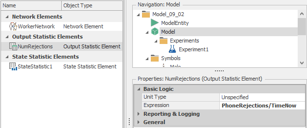
Figure 9.45: User-defined output statistic for phone rejections per hour.
As set up, our experiment evaluates scenarios containing between 1 and 5 phone lines and between 1 and 3 workers (for a total of 15 scenarios). The scenarios are sorted in order of increasing value of CustTIS — resulting in the “best” configuration(s) in terms of the time that customers spend in the system being at the top of the table. Rather than manually enumerating all scenarios within a region (as we do in Figure 9.45), we could also have used the OptQuest add-in to assist us with the identification of the “best” configuration(s) (as described in Section 9.1.1). Figure 9.46 shows the results of using OptQuest with Model 9-2. For this optimization, we used two controls and two responses to control the experiment (or, more precisely, to tell OptQuest how to control the experiment). These controls and responses are defined as follows:
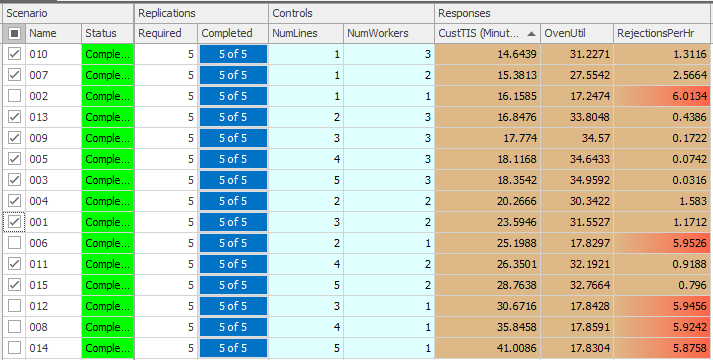
Figure 9.46: Result of using OptQuest with Model 9-2.
- NumLines (control) - the number of phone lines used. We specify a minimum of
1line and a maximum of5lines. - NumWorkers (control) - the number of workers. We specify a minimum of
1worker and a maximum of3workers. - CustTIS (response) - the time that customers spend in the system. We would like to minimize this output value (so that we can make our customers happy).
- RejectionsPerHr (response) - the number of customer call rejections per hour. We would like to keep this output value under
4(we arbitrarily chose this value). Without this service-level constraint, the optimization could minimize the customer time in system by simply reducing the number of phone lines, thereby restricting the number of customers who actually get to place an order (something the pizza shop manager would likely frown on!).
Figure 9.47 shows the control and response properties for the OptQuest-based experiment with Model 9-2. Note that we set the minimum and maximum values for the controls (NumLines and NumWorkers), we set the objective (Minimize) for the Customer TIS response and set the maximum value (4) for the RejectionsPerHr response. The results (Figure 9.46) indicate that the 1-line, 3-worker configuration results in the minimum customer time-in-system (\(14.6439\)) and an acceptable average number of rejections per hour (\(1.3116\)). In the 1-line, 1-worker configuration, there is a slightly higher customer time-in-system (\(16.1585\)), but the average number of rejections per hour violates our constraint (\(6.0134 > 4\)) — note that the Rejections/Hr cell for this configuration is highlighted in red, indicating the infeasibility. The next logical step in our analysis would be to use the Subset Selection Analysis and/or the Select Best Scenario using KN to identify the “best” configuration – we will leave this as an exercise for the reader (see Problem 4).
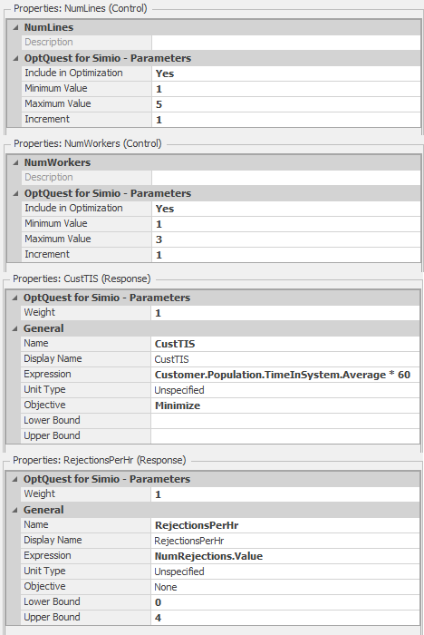
Figure 9.47: Control and response properties for the OptQuest experiment with Model 9-2.
9.3 Model 9-3: Fixed-Capacity Buffers
The final model for this chapter involves modeling an assembly line with fixed-capacity buffers between the stations. In an assembly line, items move sequentially from station to station starting at station 1 and ending at station \(n\), where \(n\) is the length of the line. Adjacent stations in the line are separated by a buffer that can hold a fixed number of items (defined as the buffer capacity). If there is no buffer between two stations, we simply assign a zero-capacity buffer (for consistency in notation). Consider two adjacent stations, \(i\) and \(i+1\) (see Figure 9.48).
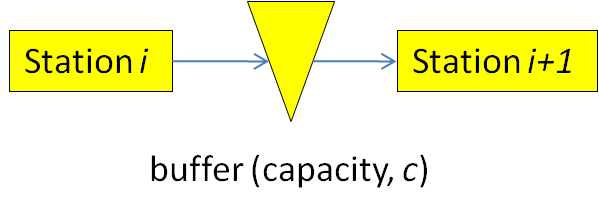
Figure 9.48: Two adjacent stations separated by a buffer.
If station \(i\) is finished working and the buffer between the stations is full (or zero-capacity), station \(i\) is blocked and cannot begin processing the next item. On the other hand, if station \(i+1\) is finished and the buffer is empty, station \(i+1\) is starved and similarly cannot start on processing the next item. Both cases result in lost production in the line. Clearly in cases where the processing times are highly variable and/or where the stations are unreliable, adding buffer capacity can improve the process throughput by reducing blocking and starving in the station. The buffer allocation problem involves determining where buffers should be placed and the capacities of the buffers. Model 9-3 will allow us to solve the buffer allocation problem (or, more specifically, will provide throughput analysis that can be used to solve the buffer allocation problem). A more detailed description of serial production lines and their analysis can be found in (Askin and Standridge 1993), but our brief description is sufficient for our needs.
Our goal for Model 9-3 is to be able to estimate the line’s maximum throughput for a given buffer configuration (the set of the sizes of buffers between the stations). Throughput in this context is defined as the number of items produced per unit time. For simplicity, our model will consider the case where stations are identical (i.e., the distributions of processing times are the same) and the buffers between adjacent stations are all the same size so that the buffer configuration is defined by a single number — the capacity of all of the buffers. Model 9-3 can be used to replicate the analysis originally presented in (Conway et al. 1988) and described in (Askin and Standridge 1993). Figure 9.49 shows the Facility view of Model 9-3.
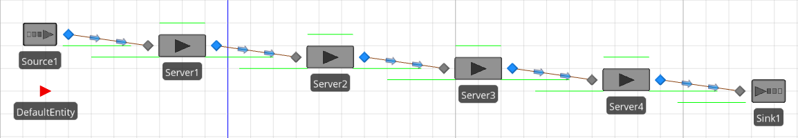
Figure 9.49: Facility view for Model 9-3.
From the Facility view, Model 9-3 looks much like Model 5-1 with three additional stations added between the Source and Sink objects. There are, however some subtle differences required to model our fixed-capacity buffer assembly line. We will discuss these changes in the following paragraphs. In addition, we will also demonstrate the use of referenced properties and the Simio Response Charts as tools for experimentation and scenario comparison.
By default, when we connect two Server objects with a Connector or Path object, entities are automatically transferred from the output node of one station to the input node of the next station once processing is complete at the first station. If the second station is busy, the transferred entity waits in a queue. When the second server is available it removes the first entity waiting in the queue and begins processing. This essentially models an infinite capacity buffer between two stations and does not model the blocking effect associated with finite-capacity buffers. Consider the simple case where we have a zero-capacity buffer (e.g., no buffer) between two stations that we model as resources. What we need instead of the default behavior is to ensure that the subsequent resource has available capacity before we release the current resource (i.e., making sure that the entity has somewhere to go before it starts going). This is described as overlapping resources in (Kelton, Sadowski, and Zupick 2015). Clearly if we have a finite-capacity buffer between the two stations, we have an analogous problem — we just need to make sure that the buffer instead of the subsequent resource has remaining capacity.
Luckily, the Simio Server object makes it fairly easy to model this type of overlapping resources situation. Figure 9.50 shows the properties for the Server1 object in Model 9-3. Our interest here is in the Buffer Capacity section of the properties and the Input Buffer and Output Buffer properties in particular. The Input Buffer for a Server object is used to hold entities that are entering the server when there is not sufficient capacity on the server resource. Similarly, the Output Buffer is used to hold entities that have completed processing on the server, but do not yet have anywhere to go. Whereas the default value for these properties is Infinite, we use a referenced property named BufferCapacity to specify the Input Buffer size and set the Output Buffer to 0. With this configuration for all of our stations, an entity can only be transferred from one Server to the next if the number of entities in the internal queue representing the input buffer of the subsequent station is less than the value of the referenced property BufferCapacity. Note also that we specified the Processing Time property using another referenced property, ProcessingTime. Using the referenced properties for the buffer capacity and processing time distributions will simplify experimentation with different line configurations (as we will illustrate below). While we don’t use them in this model, Simio’s Standard Library objects have robust support for balking and reneging with many options. These features are accessed through the Balking & Reneging Options properties (see Figure 9.50). Model 10-3 in Section 10.2 presents a use-case in detail.
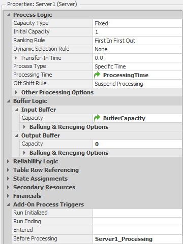
Figure 9.50: Properties for the Server1 object in Model 9-3.
Since we are using the model to estimate the maximum throughput for a line, we also need to modify the entity arrival process. As we have seen, the standard Source object will create entities using an interarrival time distribution or an arrival schedule. For our maximum throughput model, we need to make sure that there is always an entity waiting for the first station (Server1). This way, the first station will never be starved (this is equivalent to saying that there is an infinite supply of raw materials for the line). To implement this logic, we simply set the Maximum Arrivals property on Source1 to 1 (so that we will create a single entity at time zero) and we duplicate the entity when it finished processing on Server1 and send the duplicate back to the input of Server1. We accomplish this duplication and routing using the Server1_Processing add-on process for Server1. (see Figure 9.51).
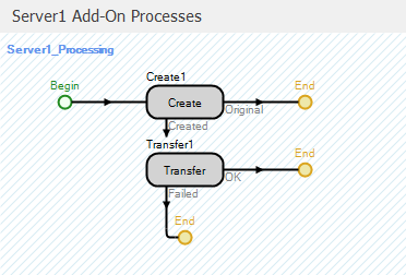
Figure 9.51: Processing add-on process for Server1.
The Create step duplicates the entity and the Transfer step connected to the Created output of the Create step transfers the entity to the node Input@server1. Since the Original output goes to the End of the process, the original entity will follow the normal path and either be transferred to the second station if there is available capacity either in Server2 or in the buffer between Server1 and Server2 or will remain on Server1 since the Output Buffer capacity is set to 0. See Problem 8 at the end of the chapter for an alternate method of maintaining the infinite supply of raw materials at the first station.
Now that the initial model is complete, we can use the model to experiment with different configurations. Figure 9.52 shows an experiment for Model 9-3. Note that since we defined referenced properties for the station processing times (ProcessingTime) and the buffer capacities (BufferCapacity), these show up as Controls in the experiment. In this experiment we defined eleven scenarios where the processing times are exponentially distributed with mean 10 minutes and the buffer capacity goes from 0 to 10 in steps of 1. For this experiment, we set the run length to 30,000 minutes and the warm-up period to 20,000 minutes. With 10,000 minutes of run time and mean processing times of 10 minutes at each station, we would expect 1,000 items to be produced in the absence of processing time variation (for a Throughput of 6 per hour). To track this, we use the DefaultEntity.Population.NumberDestroyed expression for the TotalProduced response and divided that by (Run.TimeNow-Run.WarmupPeriod) for the Throughput response (note that in this case, we could also have used Sink1.InputBuffer.NumberEntered for the number produced). For the scenarios tested the average throughput for 50 replications ranged from 3.105 with no buffers to 5.231 with 10 buffers.
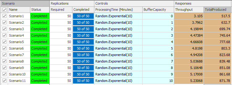
Figure 9.52: Experiment with exponentially distributed processing times for Model 9-3.
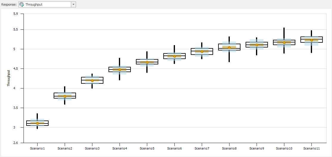
Figure 9.53: Response chart for exponentially distributed processing times for Model 9-3.
As we have previously discussed, Simio automatically tracks the busy/idle state for resources and Server objects. In fact, by default, Simio tracks the following states for Server objects:
- Starved - The server is idle and waiting for an entity
- Processing - The server is processing one or more entities
- Blocked - The server has completed processing, but the entity cannot release the server
- Failed - The server has failed
- Offshift - The server uses a schedule and is off-shift
For our serial production line with an infinite supply of items at the first server, no server failures, and no work schedules, the servers can either be processing an item (busy), starved (idle), or blocked. We can use Simio’s Status Pie chart feature to track the states of the four servers in our serial line (see Figure 9.54).
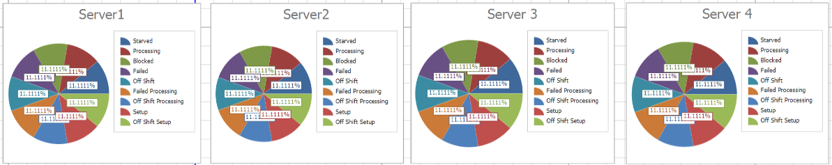
Figure 9.54: Server state status pie charts for Model 9-3.
The Status Pie charts show the percentage of time that the given server was in the respective states. Figure 9.55 shows the properties for the Status Pie charts for a new chart (left), Server1 (top right) and Server3 (bottom right). In the new chart, using the Data Source property pull-down shows the ResourceState list states for the four serves. Once you select one of these data sources (as we show for the Server1 and Server3 charts), the Expressions property is no longer active. The difference between the two charts is that the Server3 chart is attached to Server3 whereas the Server1 chart is not attached to Server1 (recall that to create an attached animation object, select the target object and use the Attached Animation ribbon rather than the standard Animation ribbon). Since the Server3 chart is attached to the Server object, the chart will “move” with the Server object in the Facility view whereas the chart for Server1 will not “move” with the Server.
Notice that the first server in the line is never starved and the last server is never blocked. This is exactly as we would expect in a model designed for assessing maximum throughput. Comparing the second and third stations, the second station has more blocking and the third station has more starving. If we had a longer line, this pattern would continue — stations nearer the start of the line experience more blocking and stations near the end of the line experience more starving.
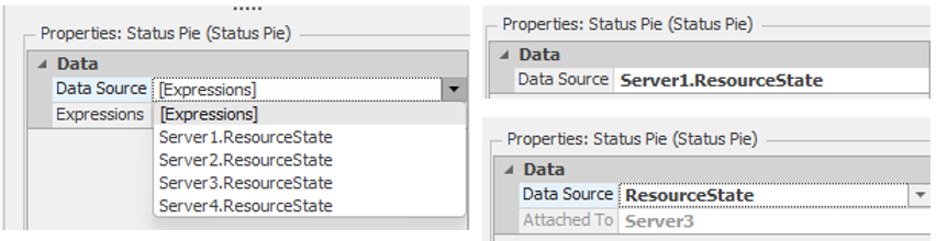
Figure 9.55: Properties for the Status Pie Charts for a new chart (left), Server1 (top right), and Server3 (bottom right).
Since we used a referenced property to specify the processing time distributions, we can easily change these in the experiment (no need to go back to the model). Figure 9.56 shows the Response Chart for an experiment similar to the one shown in Figure 9.52 except with triangularly distributed processing times with parameters (5, 10, 15) — we simply changed the referenced property values in the Controls section of the experiment. Since the variance is significantly less with the triangular distribution than with the exponential distribution, we expect the blocking and starving effect to be less for the triangular case, and we expect the throughput recovery by adding buffers to be faster (i.e., more throughput recovery with fewer buffers). All of these analysis results match our expectation as well as the results of using the methods described in (Askin and Standridge 1993) and (Conway et al. 1988).

Figure 9.56: Response chart for triangularly distributed processing times for Model 9-3.
9.4 Summary
In this chapter we’ve looked at Simio models of three systems — each involving one or more advanced simulation concepts. In addition to the modeling aspects, we also focused on the experimentation with each of these models and introduced the OptQuest simulation-based optimization add-in. Once the user defines the appropriate objective, constraints, and requirements, OptQuest “drives” the Simio experiment towards an optimal configuration of the system. We also described the ranking and selection process, by which we try to identify the “best” solution from those scenarios provided by OptQuest and demonstrated the use of Simio’s Subset Selection Analysis function and the Select Best Scenario using the KN add-in. These tools significantly simplify the general output-analysis process.
Of course we have merely scratched the surface of the applications of simulation in general and the capabilities of Simio in particular, so you should definitely consider this as the beginning rather than the end of your quest to master the use of simulation and Simio. Further, our coverage of output analysis in general, and simulation-based optimization in particular, has been extremely introductory in nature, and there is much more to be learned from other sources and experimentation.
9.5 Problems
- Modify Model 9-1 so that it includes the patient physical movement and Nurse/Aide escort functionality from Model 8-3. Compare the resource requirements with those of Model 9-1. Does including this level of detail “improve” the validity of the results? If so, why? If not, why not?
- Modify Model 9-1 to support preemption of the Doctor resource for Urgent patients. In particular, if all doctors are busy when an Urgent patient arrives, the Urgent patient should preempt a doctor from one of the other non-Urgent patients. Compare the results of the models. Would you advise that the emergency department make the corresponding change in the real system?
- In Model 9-2, we used a 1000 hour run length with no warm-up period (and gave no explanation for these settings). Do they appear reasonable? Why or why not? Could you achieve the same results with a shorter run length? Would a longer run length improve the results?
- In Section 9.2.1 we experimented with model 9-2 (manually and with OptQuest), but we did not use the Subset Selection Analysis function and/or Select Best Scenario using KN add-in to identify the “best” configuration(s) from the identified set. Do this and make any necessary adjustments to the numbers of replications required to identify the “best” configuration.
- Many pizza take-out places around these days also deliver. Modify Model 9-2 to support the delivery of customer orders. Assume that 90% of customers would like their pizzas delivered (the remaining 10% will pick them up as we assumed in Model 9-2). The pizza shop has divided the customer delivery area into four zones and a delivery person can take multiple orders on the same delivery trip if the orders come from the same zone. Table 9.3 gives the delivery time distributions for each zone and the proportion of customers from each zone. For simplicity, if a delivery includes more than one order, simply add 4 minutes to the sampled delivery time for each extra order. For example, if a delivery includes 3 orders and the originally sampled delivery time is 8 minutes, you would use \(8+4+4=12\) minutes for the total delivery time instead. For customer arrivals, processing times, and worker characteristics, use the same data as was given for Model 9-2. Develop an experiment to determine how many delivery people should be hired. Be sure to justify your solution (i.e., how you decided the appropriate number of delivery people).
- Modify the model from Problem 5 so that delivery people wait until there are at least 2 orders waiting to be delivered to a given zone before they start a delivery. Compare the results to the previous model. Is this a good strategy? What about requiring at least 3 orders?
- Consider a six-station serial manufacturing line similar to the assembly line in Model 9-3. As with Model 9-3, there are finite-capacity buffers between each pair of stations (assume that the first station is never starved and the last station is never blocked). The difference in the current system is that the stations are not identical in terms of the processing time distributions and some are subject to random failures. The processing time distributions and failure data are given in Table 9.4 (note that the Lognormal distribution parameters (4, 3) for Station 5 are the mean and standard deviation of the generated random variates while the arguments for the Random.Lognormal() function are the mean and standard deviation of the underlying normal random variates – see the Simio Help for details about the required conversion). Develop a Simio model of the serial line and create an experiment that will find a “good” allocation of 30 buffer slots. For example, one allocation would be \([6, 6, 6, 6, 6]\) (6 slots between each pair of stations). The objective is to maximize the line throughput. Does your experiment find the guaranteed optimal buffer allocation? If so, why? If not, why not?
- Modify Model 9-3 to use the
On EventArrival Mode property for the Source object to create new entities for the first station rather than using the add-on process associated with the Server1 object as described in Section 9.3. - In the OptQuest-based experiment described in Section 9.2.1, we minimized the customer time in system subject to a service level constraint. However, we didn’t consider staffing costs. As an alternative, develop a single “total cost” metric that incorporates customer waiting time, worker costs, and customer service. Add the total cost metric as an output statistic and use OptQuest to find the optimal configuration(s).
- Model 9-2 uses a pooled employee strategy for taking orders, making pizzas and boxing pizzas. Develop a model that uses a dedicated employee strategy (i.e., each employee is dedicated to a task) and compare the results with those of Model 9-2. Under what conditions is one strategy preferred over the other? Justify your answer with experimentation.
| Zone | Proportion | Delivery Time Distribution |
|---|---|---|
| 1 | 12% | Triangular(5, 12, 20) |
| 2 | 30% | Triangular(2, 7, 10) |
| 3 | 18% | Triangular(8, 15, 22) |
| 4 | 40% | Triangular(6, 10, 15) |
| Num | Processing Time | Uptime | Time to Repair |
|---|---|---|---|
| 1 | Triangular(3,6,9) | Exponential(360) | Exponential(20) |
| 2 | Exponential(3) | Exponential(120) | Triangular(10,15,20) |
| 3 | Erlang(6,3) | Exponential(300) | Exponential(5) |
| 4 | Triangular(2,7,12) | N/A | N/A |
| 5 | Lognormal(4,3) | Exponential(170) | Triangular(8,10,12) |
| 6 | Exponential(6) | N/A | N/A |