Simio and Simulation: Modeling, Analysis, Applications - 7th Edition
Chapter 7 Working With Model Data
There are many different types of data used in a model. So far we’ve largely entered our data directly into the properties of Standard Library objects. For example, we entered the mean interarrival time directly into a Source object and entered the parameters of the processing-time distribution directly into a Server object. While this is fine for some types of data, there are many cases where other mechanisms are necessary. Specific types of data, such as time-varying arrival patterns, require a unique data representation. In other situations, the volume of data is large enough that it’s necessary to represent the data in a more convenient form, and in fact even import the data from an external source. And in situations where the analyst using the model may not be the same as the modeler who builds the model, it may be necessary to consolidate the data rather than having them scattered around the model. In this chapter we’ll discuss many different types of data and explore some of the Simio constructs available to represent those types of data best.
7.1 Data Tables
A Simio Data Table is similar to a spreadsheet table. It’s a rectangular data matrix consisting of columns of properties and rows of data. Each column is a property you select and can be one of about 50 Simio data types, including Standard Properties (e.g., Integer, Real, Expression, Boolean), Element References (e.g., Tally Statistic, Station, Material), or Object References (e.g., Entity, Node List). Typically, each row has some significance; for example it could represent the data for a particular entity type, object, or organizational aspect of the data.
Data tables can be imported, exported, and even bound (see Section 7.1.7) to an external file. They can be accessed sequentially, randomly, directly, and even automatically. You can create relations between tables such that an entry in one table can reference the data held by another table. In addition to basic tables, Simio also has Sequence Tables and Arrival Tables, each a specialization of the basic table. All of these topics will be discussed in this section.
While reading and writing disk files interactively during a run can significantly slow execution speed, tables hold their data in memory and so the data can be accessed very quickly. Within Simio you can define as many tables as you like, and each table can have any number of columns of different types. And you can have as many rows as needed - limited only by your system memory. You’ll find tables to be valuable in organizing, representing, and using your data as well as interfacing with external data.
7.1.1 Basics of Tables
A data table is defined using the Table Tools panel in the Data window (see Figure 7.1). Note that the Table Tools panel includes two ribbons – Schema and Content – that separate the tools related to editing table structure from tools related to table content. To add a new table you click on Add Table in the Tables section of the Schema ribbon. Once you’ve added a table you can rename it and give it a description by clicking on the tab for the table and then setting the table properties in the Property window.
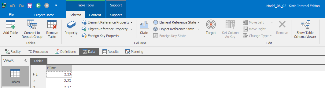
Figure 7.1: Table Tools Panel for Model 6-2.
Tip: If you add multiple tables, each one has its own tab. And if you have many tables, you will see a pull-down list on the right end of the tab row listing the tabs currently out of view. Recall our discussion in Section 4.1.8 about configuring window placement. That can be particularly handy when working with data tables.
To add columns to a table you select a table to make it active and then click on property types under Standard Property, Element Reference, Object Reference, or Foreign Key. A table column is typically represented by the Standard Properties illustrated in Table 7.1.
| Property Type | Description |
|---|---|
| Boolean | True (1 or non-zero) or False (0) |
| Color | A property for graphically setting color |
| Changeover Matrix | A reference to a changeover matrix |
| Date Time | A specific day and time (7:30:00 November 18, 2010) |
| Day Pattern | A reference to a Day Pattern for a schedule |
| Enumeration | A set of values described in a pre-defined enumeration |
| Event | Event that triggers a token release from a step |
| Expression | An expression evaluated to a real number (1.5+MyState) |
| Integer | An integer number (5 or -1) |
| List | A set of values described in a string list |
| Rate Table | A reference to a rate table |
| Real | A decimal number (2.7 or -1.5) |
| Schedule | A reference to a schedule |
| Selection Rule | A reference to a selection rule |
| Sequence Destination | References an entry/exit node |
| Sequence Number | Specify an integer or dot-delimited sequence of integers |
| Sequence Table | A reference to a sequence table |
| State | A reference to a state |
| String | Textual information (Red, Blue) |
| Table | A reference to a data table or sequence table |
| Task Dependency | Define predecessor or successor relationships for a task |
Use an Object Reference when you want a table to reference an object instance or list of objects such as an Entity, Node, Transporter, or other model object. Likewise use an Element Reference if you want a table to reference a specific element like a TallyStatistic or Material. As you are defining the name, positioning, data type, and other properties of each column, you are defining the Schema of the data table. Simio allows you to define any schema you need – you might choose a schema for convenience accessing in Simio, or you might define a schema matching that of an external file so you can import and use that external data without converting or transforming it.
In version 16.256, Simio introduced the Histogram Tool for data tables (see Figure 7.2 for an example). The Histogram Tool is accessed from the Content section of the Table Tools ribbon and can generate standard frequency histograms (along with basic descriptive statistics) from any of the numeric type columns in the selected table. The generated histogram windows are non-modal, so multiple histogram windows can be open simultaneously for side-by-side comparison. While the generated histograms are fairly basic and the tool does not support customization (e.g., bin-size specification), the data can easily be exported (see Section 7.1.7) and accessed using a statistical analysis tool (like Minitab) for more detailed analysis.
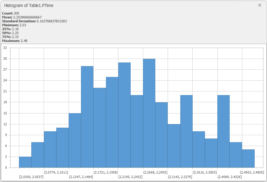
Figure 7.2: Histogram for PTime1 from Model 6-2.
7.1.2 Model 7-1: An ED Using a Data Table
Let’s illustrate these table concepts by representing the data for a simple healthcare example. Consider an emergency department (ED) that has some known data concerning how patients of various severities are processed. Specifically, we have four patient types, their priority value, and their typical treatment time as given in Table 7.2.
| Patient Type | Priority | Treatment Time (Minutes) |
|---|---|---|
| Routine | 1 | Random.Triangular(3,5,10) |
| Moderate | 2 | Random.Triangular(4,8,25) |
| Severe | 3 | Random.Triangular(10,15,30) |
| Urgent | 4 | Random.Triangular(15,25,40) |
The first steps in building our model involve defining the model entities and the data table:
Load Simio and start a new model as we’ve done before. The first thing we’ll do is drag four instances of
ModelEntityinto the model facility view. Click on each one and use the properties or theF2key to rename them toRoutine,Moderate,Severe, andUrgent, respectively.Let’s take a minute to animate those entities a little better, so that we can tell them apart. Follow the same procedure described in Section 4.8. Although all entities will use the default entity symbol, we can tell them apart by giving each entity instance a different color. Zoom in so you can see your new symbols clearly. Click on the
Moderateentity. On the right side of the Symbols ribbon is aColorbutton. Clicking the lower half of the color button will display a color pallet. Select a yellow color and then apply it toModerateby clicking on the entity instance symbol. Repeat this procedure to apply a light blue to theSeverepatients and Red to theUrgentpatients. We’ll leaveRoutinewith the default color.Next, let’s create the data table. Select the
Datatab just under the ribbon, and then select theTablespanel on the left if it’s not already selected. The Table ribbon will appear, although many items will be unavailable (grayed out) because we don’t yet have an active table. Click on theAdd Data Tablebutton to add a blank table, then click on the Name property in the properties window and change the name toPatientData(no spaces are allowed in Simio names).Now we’ll add our three columns of data. Our first column will reference an entity type (an object), so click on
Object Referenceon the ribbon and then selectEntityfrom that list. You’ve now created a column that will hold an Entity Instance. Go to the Name property (not the Display Name property) in the properties window and change it toPatientType. Our second column will be an integer, so click onStandard Propertyin the ribbon and selectInteger. Go to the Name property and rename it toPriority. Finally, our third column will be an expression so click onStandard Propertyin the ribbon and selectExpression. Go to the Name property and rename it toTreatmentTime. Since this represents a time, we need a couple of extra steps here: In the Value category of the properties window, specify a Unit Type ofTimeand specify Default Units ofMinutes.Now that we have the structure of the table, let’s add our four rows of data. You can add the data from Table 7.2. You can enter the data a row at a time or a column at a time; here we’ll do the former. Click on the upper left cell and you’ll see a list containing our four entity types. (If you don’t see that list, go back two steps.) Select
Routineas the Patient Type for row 1. Move to thePrioritycolumn, type1and press tab or enter and you’ll be moved to theTreatmentTimecolumn. Here we’ll type in the expression from Table 7.2,Random.Triangular(3,5,10). Tip: If the values of your data are partially hidden, you can double click on the right edge of the column name and it will expand to full width. Move to the next row in the PatientData table and follow a similar process to enter the remaining data from Table 7.2.
When you’re finished your table should look similar to Figure 7.3.
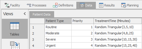
Figure 7.3: Model 7-1 ED basic patient data in Simio table.
We’ve now defined the patient-related data that our model will use. In the next section, we’ll demonstrate how to access the data from the table.
7.1.2.1 Referencing Data Tables
Table data can be used by explicitly referencing the table name, the row number, and the column name or number using the syntax TableName[RowNumber].ColumnName or the syntax TableName[RowNumber,ColumnNumber]. We could continue building our model now using that syntax to reference our table data. For example, we could use PatientData[3].TreatmentTime to refer to the treatment time for a Severe patient. While using this syntax is useful for referencing directly into a cell of a table, we often find that a particular entity will always reference a specific table row. For example in our case, we’ll determine the row associated with a patient type, and then that entity will always reference data from that same row. You could add your own property or state to track that, but Simio already builds in this capability. The easiest method to access that capability is by setting the properties in the Table Row Referencing category of the Source object.
If we had a separate arrival stream for each of our four patient types, we’d probably use this technique. We’d have a source object to create each patient type. Figure 7.4 illustrates how the source object for Severe patients could be configured by specifying the table name and an explicit row number. Once you’ve made this association between an entity and a specific row in a table, you can use a slightly simpler syntax to reference the table data: TableName.ColumnName because the row number is already known. For example, we could now use PatientData.TreatmentTime to refer to the treatment time for any patient type.
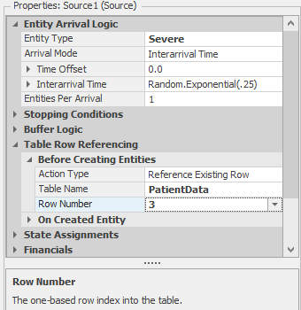
Figure 7.4: Associating an entity with an explicit row in a table.
7.1.2.2 Selecting Entity Type
Before we finish our model, we’ll explore one more aspect of tables. It’s very common to have data in a table where each row corresponds to an entity type, as we have in our model. It’s also common to have the entity type be selected randomly. Simio allows you to do both within the same construct. You can add a numeric column to your table that specifies the relative weight for each row (or entity type). Then you can specify that you’ll randomly select a row based on that column by using the function TableName.ColumnName.RandomRow.
Let’s follow a few final steps to complete our model.
- In our ED, historical information suggests that our patient mix is
Routine(40%),Moderate(31%),Severe(24%), andUrgent(5%). We need to add this new information to our table. Return to the Data tab and the Tables panel. ClickStandard Propertyand selectReal. Go to the Name property and rename it toPatientMix. Then add the above data to that new column. When you’re finished your table should now look like Figure 7.5. Note that, as noted in Section 5.2, the values in the Patient Mix column are interpreted by Simio only in relation to their relative proportions. While we entered the values here thinking of the percent of patients of each type, they could have equivalently been entered as probabilities (0.40, 0.31, 0.24, 0.05), or as any other positive multiple of the values we used (e.g., 4000, 3100, 2400, 500).
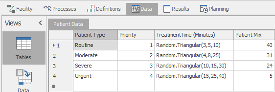
Figure 7.5: Model 7-1 ED Enhanced patient data in Simio table.
- Now we can continue building our model. The last change we made allows us to have a single Source that will produce the specified distribution of our four patient types. Place a Source in your model and specify an Interarrival Time of
Random.Exponential(4)and units ofMinutes. Instead of specifying one patient type in the Entity Type property with a specific row number as we did in Figure 7.4, we’ll let Simio pick the row number and then we’ll select the Entity Type based on the PatientType specified in that row. We must select the table row before we create the entity; otherwise the entity would already be created by the time we decide what type it is. So in the Table Reference Assignment, Before Creating Entities category, we will specify the Table Name ofPatientDataand the Row Number ofPatientData.PatientMix.RandomRow. After the row is selected, the Source will go to the Entity Type property to determine which Entity Type to create. There we can selectPatientData.PatientTypefrom the pull-down list. This is illustrated in Figure 7.6.
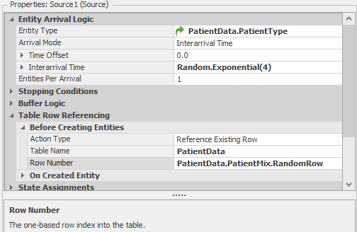
Figure 7.6: Selecting an entity type from a table.
- Completing our model is pretty painless. Add a Server, set its Initial Capacity to
3, and specify a Processing Time ofPatientData.TreatmentTime. We’re using the data in the table for this field, but note that we’re using the short reference method. Since no explicit row is specified, we’re telling Simio to use the row that’s already associated with each specific entity. When an entity of type Routine arrives, it will use row one and a treatment time sampled from the distributionRandom.Triangular(3,5,10). However, when an entity of type Severe arrives, it will use row three and a treatment time sampled from the distributionRandom.Triangular(10,15,30). Add a Sink, then connect Source to Server and Server to Sink with Paths. Your model should look something like Figure 7.7.
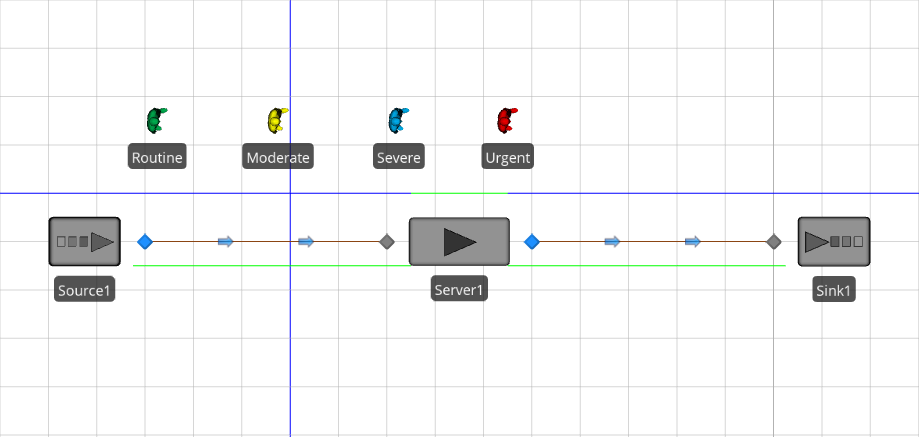
Figure 7.7: Model 7-1 Completed ED model.
Before enhancing our model, we’ll do a small verification step so that we’ll be confident that we’ve correctly implemented the data table. Using the proportions of patient types and the expected service times for each patient type, we can compute the overall expected service time (11.96 minutes). With the overall arrival rate of 15 patients/hour, we expect a steady-state server utilization of 99.64%. We ran Model 7-1 for 25 replications of length 200 days with a 25-day warmup period and the resulting average scheduled utilization was \(99.67\% \pm 0.1043\) (the 95% confidence interval half-width). This illustrates an important point about model verification — it’s often much easier to verify the model as you build it rather than waiting until the model is “finished.” Since our sampled utilization matched our expectation quite well, we’re now confident that we’ve properly implemented the patient data table and can move on to our model enhancements.
7.1.3 Sequence Tables
A sequence table is a special type of data table used to specify a sequence of destinations for an entity. In a manufacturing job shop, this sequence might be the stations or machines that must be visited to complete a part (e.g., Grinding, Polishing, Assembly, Shipping). For a transportation network, the sequence might be a series of stops in a bus route (e.g., MainStreet, FifthStreet, NinthStreet, Uptown).
You create a sequence table in the Tables panel of the Data Window just like for normal data tables, but use the Add Sequence Table button. This will create the table and automatically add a column named Sequence for specifying a routing sequence for an entity. This required column is the major difference between a normal table and a sequence table. In most other ways everything that applies to a data table also applies to a sequence table. Just as the properties (columns) of a table can be used however you wish, the same is true in sequence tables. Also you can reference these values the same way you’d reference the values in any other table (e.g., TableName.PropertyName).
There are actually two different ways of configuring sequence tables: simple sequence tables and relational sequence tables. Simple sequence tables are preferred when you have a somewhat isolated use of a single sequence. For example if you have only one sequence or entity type in use. Relational tables have the advantage of more easily supporting the more complex use of sequences that you might encounter with multiple entities following different sequences through the same objects. They’re both used in the same way, but differ in how the tables are configured. We’ll start by explaining how to configure and use simple sequence tables.
7.1.3.1 Simple Sequence Tables
Each simple sequence table defines one routing plan. If you have multiple routing plans (e.g., several bus routes), then each would be defined in its own sequence table. Each row in the sequence table corresponds to a specific location. The data items in that row are usually used for location-specific properties, for example the processing time, priority, or other properties required at a particular location.
After your sequence table has been created, you must create an association between the entity and the sequence table (in other words, you need to tell the entity which sequence to follow). There are various ways to do that, but the easiest is to do so on an entity instance you’ve placed in a model. It will have a property named Initial Sequence in its Routing Logic category. Specify the sequence table name in this property. The entity will start at row one in this sequence table and work its way through the rows as stations are visited. Although this happens automatically, it’s possible to change the current row, and in fact even change the sequence being followed. This can be done at any time using the SetRow step in an add-on process.
At this point the astute reader (that’s you, we hope) will be asking “But how does the entity know when to move to the next step in its sequence?” You must tell the entity when to go to the next step in its sequence. The most common place to do that is in the Routing Logic category of a Transfer Node (recall that the outbound node from every Standard Library object is a Transfer Node). Here you would specify that the Entity Destination Type is By Sequence. This causes three things to happen:
The next table row in the entity’s sequence table is made current.
The entity’s destination is set to the destination specified in that row.
Any other table properties you’ve specified (e.g., ProcessingTime) will now look to the new current row for their values.
Because you’re explicitly telling the entity when to move to the next sequence, you also have the option to visit other stations in between sequences if you choose — simply specify the Entity Destination Type as anything other than By Sequence (e.g., Specific). You can do this as many times as you wish. The next time you leave an object and you want to move sequentially, just again use By Sequence and it will pick up exactly where you left off.
7.1.3.2 Relational Sequence Tables
Many of the above concepts are the same for relational sequence tables. Relational sequence tables are used in much the same way, but configured a bit differently. One difference is that you can combine several different sequences (e.g., the set of visitations for a particular entity) into a single sequence table. And instead of setting the sequence to follow on the entity instance (using the Initial Sequence property), you can provide that information in another table. Both of these capabilities are accomplished by linking a main data table with a relational sequence table using special columns identified as Key and Foreign Key. The basics of using relational tables for sequences will be demonstrated in Model 7-2. A more complete discussion of relational tables can be found in Section 7.1.6.
7.1.4 Model 7-2: Enhanced ED Using Sequence Tables
Let’s embellish our previous ED model (Model 7-1) by describing the system in a little more detail. All patients first visit a sign-in station, then all except the Urgent go to a registration area. After being registered they’ll go to the first available examination room. After the examination is complete the Routine patients will leave, while the others will continue for additional treatment. Urgent patients visit the sign-in, but then go to a trauma room that’s equipped to treat more serious conditions. All Urgent patients will remain in the trauma room until they’re stabilized, then they’re transferred to a treatment room, and then they’ll leave.
You may recall that when we started Model 7-1, the first thing we did was place the entities. More generically, we started by placing into the model the objects that we’d be referencing in the table. We’ll do that again here. Since Sequence Tables mainly reference locations (more specifically, the input nodes of objects), we’ll start by placing the Server objects that represent those locations. Then we’ll build our new table, then return to add properties to our model.
Start with Model 7-1. Delete the path between the Server and the Sink as we’ll no longer need it. Likewise, go to the properties of Server1, right click on
Processing Time, and selectReset.Double click on the Standard Library
Serverand then click four times in the model to place four additional servers. HitEscapeor right click to exit the placement mode. Name the five servers that you now have asSignIn,Registration,ExamRooms,TraumaRooms, andTreatmentRooms. Add an additional Sink. Name the two sinksNormalExitandTraumaExit.Move to the
DataWindow and theTablespanel. We’ll start by designating our existing PatientType column as a unique Primary Key so that our sequences table can reference this. Select thePatientTypecolumn and click onSet Column as Keyin the Ribbon. At this point we can also delete theTreatmentTimecolumn — in a few moments we will replace it with a new location-specific ServiceTime column specified in the Treatments table. Click on theTreatmentTimecolumn heading, then click onRemove Columnin the ribbon.Now we can create our Sequence table. Click on
Add Sequence Table. Click in the properties area of the sequence table and set the name toTreatments. You will see that one column namedSequence, for the required locations, is automatically added for you.We need to add another column to identify the treatment type. Click on
Foreign Key. This will create a column that uniquely identifies the specific treatment type. In our case the treatment type corresponds exactly to the PatientType in the PatientData table. Go to the properties of this new column and name itTreatmentType. Because it’s a foreign reference, that means that it actually gets its values from somewhere else. The Table Key property specifies from where the Treatment Type value comes. SelectPatientData.PatientTypefrom the pull down list.We have one final column to add to our Treatments table — the processing time. Click on
Standard Propertyand selectExpression. This will create a property into which you can enter a number or expression to be used while at that location. Since that value has slightly different meanings at the different locations, we’ll go to the properties window and change the Name (not the Display Name) to a more genericServiceTime. Since this represents a time, in the Value category of the ServiceTime properties, we want to specify that Unit Type isTimeand that Default Units isMinutes.Before we enter data into our table, there’s one more thing we can change to make data entry easier. If you look at the pull down list in the first cell under Sequences, you’ll see a list of all of the nodes in your model because Sequences allow you to specify any node as a destination. This is valuable when you have stand-alone nodes as potential destinations, but our model doesn’t have any of those. We can take advantage of an option to limit the list to just input nodes at objects, and in fact that option just displays the object name to make selection even simpler. Click on the
Sequencecolumn, then go to the properties and change Accepts Any Node toFalse. Now if you look at that same pull-down list you’ll see a shorter and simpler list.Let’s enter our treatment data. In row 1, select
SignInfrom the pull-down list under Sequence. Then selectRoutinefrom the pull-down list under Treatment Type, then enter2for the Service Time. Continue entering data for additional rows until your table looks like Figure 7.8.
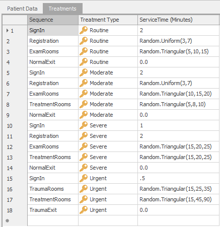
Figure 7.8: Model 7-2 Relational sequence table to define Treatments.
Now that we’ve entered our data (whew!), we can move back to the Facility window and finish our model.
Recall from the general discussion above that we must specify on each outbound node if the departure is to follow a sequence. Click on the blue TransferNode on the output side of the Source. In the routing Logic category change the Entity Destination Type to
By Sequence. You could repeat this process for each outbound node, but Simio provides a shortcut. In our case all movements will be by sequence, so we can change them all at once. Click on any blue node, then Ctrl-click one at a time on every other blue node (you should have six total). Now that you’ve selected all six transfer nodes you can change the Entity Destination Type of all six nodes at once.Connect the nodes with all the paths that will be used. If you add unnecessary paths, it adds clutter, but does no harm — for example a path from Registration to TraumaRooms would never be used because Urgent patients bypass Registration.
We’ve not yet told the Servers how long a patient will stay with them — the Process Time property on the servers. For all servers, the answer will be the same — use the information specified in the sequence associated with that specific patient and the sequence step that’s active. The expression for this is in the form
TableName.PropertyName, or specifically in this case it’sTreatments.ServiceTime. Enter that value for Process Time on each server. Note that the entity (the patient) carries with it current table and row associations.Some patients are more important than others. No, we’re not talking about politicians and sports stars, but rather patient severity. For example, we don’t want to spend time treating a chest cold while another patient may be suffering from a severe heart attack. We already have patient priority information in our patient table, but we need to change the server-selection priority from its default First In First Out (FIFO). For each server you need to change the Ranking Rule property to
Largest Value First. That will expose a Ranking Expression property that should point to our table:PatientData.Priority. This will guarantee that an Urgent patient (priority 4) will be treated before all other patients (priorities 1-3).Each of our servers actually represents an area of the ED, not just a single server. We need to indicate that by specifying the Initial Capacity for each Server. Click on each server and complete the Initial Capacity field as indicated in Table 7.3. The green line above each server displays the entities currently in process. You should extend those lines and make them long enough to match the stated capacity. Likewise, the line to the left of each server displays patients waiting for entry. Those lines may also need to be extended. You can do this while the model is running to make it easier to set the right size.
| Service Area | Initial Capacity |
|---|---|
| SignIn | 1 |
| Registration | 3 |
| ExamRooms | 6 |
| TreatmentRooms | 6 |
| TraumaRooms | 2 |
If you’ve followed all of the above steps you’ve completed the model. Although you’ve probably arranged your objects differently, it should look something like Figure 7.9 (shown with Browse window collapsed).
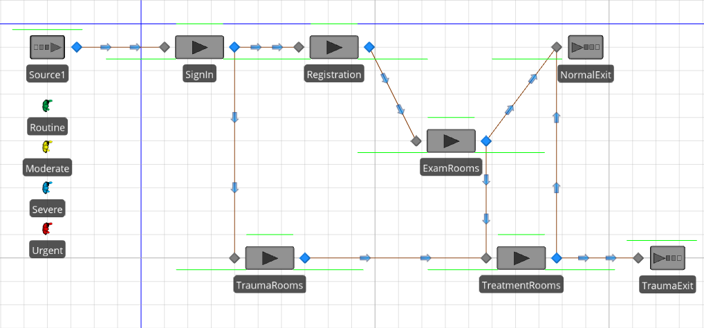
Figure 7.9: Model 7-2 completed ED model with sequences.
Continuing our strategy of verifying our models as we go, we’ll use a queueing-network model (shown in Figure 7.10) to approximate the expected steady-state utilization of the five servers. Table 7.4 gives the expected utilizations from the queueing-network model along with the results from Model 7-2 (based on 25 replications of length 200 days with 25-day warmup). Clearly our experimental results are in line with our expectations so we’re confident about our model and can continue enhancing it.
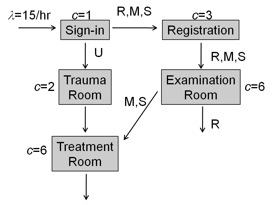
Figure 7.10: Queueing-network model for the ED model with sequences.
| Server | Expected Utilization | Simulation Results |
|---|---|---|
| Sign-in | 0.4213 | 0.4214 \(\pm\) 0.0797 |
| Registration | 0.3358 | 0.3359 \(\pm\) 0.0678 |
| Trauma Rooms | 0.1563 | 0.1567 \(\pm\) 0.1113 |
| Examination Rooms | 0.5604 | 0.5608 \(\pm\) 0.1090 |
| Treatment Rooms | 0.4032 | 0.4038 \(\pm\) 0.1132 |
7.1.5 Arrival Tables and Model 7-3
One more type of table that we’ve not yet discussed is an Arrival Table. This is used with the Arrival Mode property of the Source object to generate a specific set of arrivals as specified in a table. The arrivals can be either stochastic or deterministic.
While deterministic arrivals are uncommon in a typical stochastic simulation model, two important applications are Scheduling and Validation. In a scheduling-type application, you have a fixed set of work to get done, and you want to determine the best way to process the items to meet system objectives. Similarly, one validation technique is to run a known set of events through your model and analyze any differences between the actual results and your model results. In either case you could use an arrival table to represent the incoming work or other activities like material deliveries. Each entry in the table corresponds to an entity that will be created.
The same table can be used for stochastic arrivals by taking advantage of two extra properties in the Source object. Arrival Time Deviation allows you to specify a random deviation around the specified arrival time. Arrival No-Show Probability allows you to specify the likelihood that a particular arrival may not occur. These properties make it easy to model anticipated arrivals of items like patients (as we will illustrate below), incoming materials, and trucks for outbound deliveries. Note that, Like other model aspects, these stochastic features are disabled when the model is run in deterministic mode by selecting the Disable Randomness option in the Advanced Options on the Run tab.
Any table can be used as an Arrival Table as long as it contains a column with a list of arrival times. Arrival tables are not limited just to providing an arrival time; the rest of the table could have a full set of properties and data to determine expected routing and expected performance criteria. Let’s explore how we could use an arrival table with our ED model. We’ll add a table with an arrival time and patient type onto Model 7-2.
Go to the Tables Panel of the Data window and click
Add Data Table. Name itTestArrivals.Click on
Standard Propertyand selectDate Time. Also, name this propertyArrivalTime.Click on
Foreign Key. This will add a property that will determine the arrival type. Name itPatientType, set the Table Key toPatientData.PatientType, and the default value toRoutine. Use of the Foreign Key links this column to the other data tables we’ve already entered — no extra effort is necessary. In fact, we can eliminate the Table Reference Assignments that we previously entered on the Source object.Now we can enter some sample data, perhaps the actual patient arrivals from yesterday. Enter the data as shown in Figure 7.11. If you found it more convenient to enter the time as an elapsed time from the start of the simulation (midnight), that’s also possible. Instead of creating a Date Time property, create a property of type
Realand specify that it’s aTimeand your preferred units (e.g.,Minutes). It’s not necessary that the entries be in strict arrival time order. The records will be sorted by increasing time before they’re created.
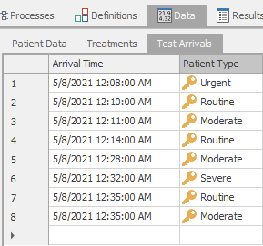
Figure 7.11: Sample arrival table.
- To trigger use of this table we must specify it on our Source. For the Arrival Mode property, select
Arrival Table. The Arrival Time Property is where you specify the table and property name that will determine the arrivals — selectTestArrivals.ArrivalTimeas shown in Figure 7.12.
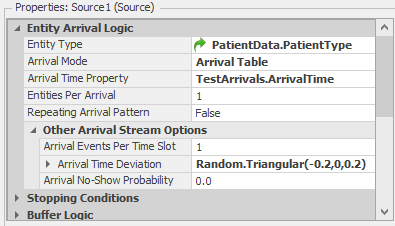
Figure 7.12: Using Arrival Tables with the Source object.
- Also on the Source, we will specify an Arrival Time Deviation of
Random.Triangular(-0.2,0,0.2)to support random arrival times. This indicates that each individual patient may arrive up to 0.2 hour early or up to 0.2 hour late (i.e., within 12 minutes of the scheduled time).
7.1.6 Relational Tables
As the name might imply, Relational Tables are tables that have a defined relationship to each other rather than existing independently. These relationships are formed by using the Table Key and Foreign Key capabilities. The Set Column As Key button allows you to indicate that the highlighted column may be referenced by another data table. This button makes that column a Key for this table and is what links the tables together. This column must have exactly one instance of each key value — none of the key values may be repeated. However, you may have multiple columns that are Key in a single table as long as each one contains a set of unique values.
Any other table, potentially multiple tables, may link to the main table by including a column of type Foreign Key that specifies the main table and its Table Key. Once that link is created, you can use any column of any linked table without having to traverse the link explicitly. For example, in Model 7-2 our PatientData table specified PatientType as a Key and that key contained four unique values. We then created our Treatments sequence table, which used that PatientType in a Foreign Key column. When we associated an entity with a particular row in PatientData, it was automatically associated with a set of related rows in the Treatments table and allowed us to use the values in Treatments.ServiceTime.
Relational tables include a Master-Detail view, which allows the relationships between various tables to be seen. For those tables that have a column that’s designated as a Key, you can see a detail view that’s a collection of rows pointing to a specific keyed row in a table. The small + sign in front of the row indicates that the detail view is available. When the + is pressed, it will show those portions of the related table specific to the entry that was expanded. We can see this if we go back to Model 7-3. If you look at the PatientType table, each PatientType entry is preceded by a +. If you press the + in front of the Moderate patient type you’ll see something like Figure 7.13.
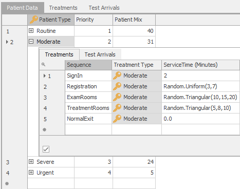
Figure 7.13: Master-Detail view of a relational table.
Under the Treatments tab, it displays all of the associated rows in the Treatments table. In this case it’s showing you all of the locations and data associated with the treatment sequence for a Moderate patient. You’ll notice that there is also a TestArrivals tab. On that tab you’ll find the data for all of the Moderate arrivals specified in the TestArrivals table. Click on the - to close the detail view and you can open and close the different keys independently.
The Table Schema Viewer, introduced in Simio version 17.261, generates a basic Entity Relationship Diagram for the data tables in a model (see Figure 7.14 shows the ERD for Model 7-3). The ER Diagram shows the data table structures, highlighting the key columns (PatientData.PatientType, in this case) and the related columns (Treatments.TreatmentType, in this case). The 1 and * symbols indicate that each PatientType row in the PatientData table can have one or more related rows in the Treatments table (a 1-to-many relationship). The Table Schema Viewer is accessed from the Schema section of the Table Tools ribbon.
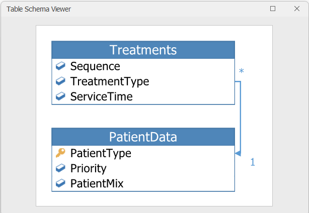
Figure 7.14: Table Schema Viewer for Model 7-3.
Relational tables provide a very powerful feature. They allow you to represent your data set efficiently and reference it simply. Moreover, this feature is very useful in linking to external data. For the same efficiency reasons, you may often find that the external data needed to support your simulation is available in a relational database. You can represent the same relationships in your data tables.
7.1.7 Table Import/Export
We trust that by this point you’ve begun to appreciate the value and utility of tables. For small amounts of data like we’ve used so far, manually entering the data into tables is reasonable. But as the volume of data increases, you’ll probably want to take advantage of the file import and export options.
You can export a table to a comma-separated-value (CSV) file by clicking on Save to CSV in the Content ribbon menu. This is useful to create a properly formatted file when you first use it or simply to write an existing table to a file for external editing (e.g., in Excel) or for backup. Figure 7.15 illustrates the interface using the previously completed Model 7-3 as an example. On the right side of the ribbon is the Save to CSV button.
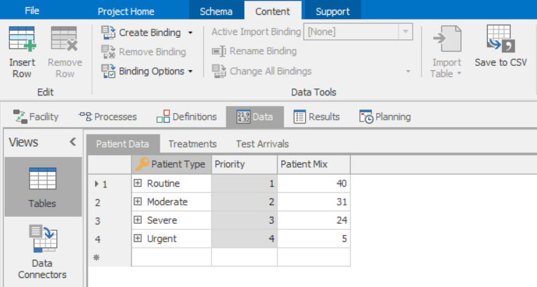
Figure 7.15: Data connectors and bindings interface.
You can also import/export the data from CSV, Excel, or many common database file formats into and out of the table by using the data connectors and binding features. Data Connectors establish the file name and any other parameters necessary to read or write the file. Binding (specifically the Create Binding button) allows you to bind a table to one or more data connectors. Both of these buttons are illustrated in Figure 7.15. The currently available importing binding types are illustrated in Figure 7.16.
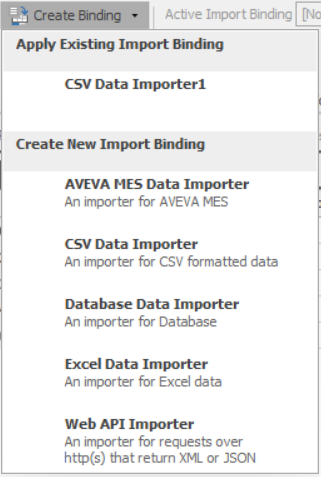
Figure 7.16: Built-in types of bindings.
Before you can import or export you must first bind the table to the external file, but the binding and the data connector can be created in any order. For example you might first select each table and create a binding, then go to the data connectors and specify the file names and parameters used with each data connector. Figure 7.17 illustrates the data connector parameters for a CSV connector.
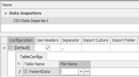
Figure 7.17: CSV data connector parameters.
Once you have bound the table to a specific file, you may also specify the Binding Options (Figure 7.18). This provides you the option of importing the data manually (only when you click the Import button) or automatically each time you start a model run. The latter is desirable if the data collection is something that changes frequently like initialization to current system status. Other more advanced options are also available.
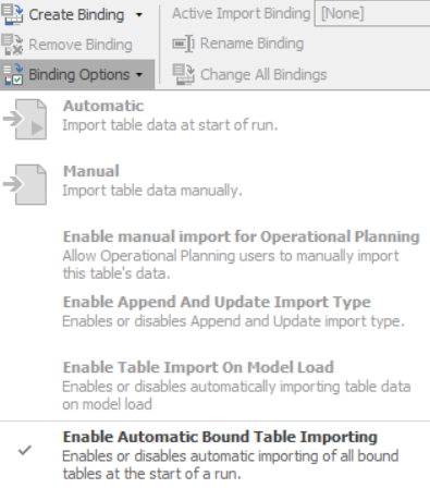
Figure 7.18: Binding options to control imports and exports.
A similar procedure and set of options are available to export tables to files. This is particular useful when you want to edit the data outside of Simio (e.g., export, edit, then re-import), record an enduring copy of your data table, or export the results of a run. See the Importing and Binding to Tables topic in Simio Help for details about setting up and configuring the bindings.
7.2 Schedules
As noted in Section 5.1.5, any object can be a resource. Those resources have a capacity (e.g., the number of units available) that may possibly vary over time. As introduced in Section 5.3.3, one way to model situations where the capacity of an object varies over time is to use Schedules. Many objects support following a Work Schedule that allows capacity to change automatically over time. The numerical capacity is also used to determine if a resource is in the On-Shift state (capacity greater than zero) or Off-Shift state (capacity equals zero). For some objects (i.e., Worker), capacity can be only either 0 (off-shift) or 1 (on-shift). For most objects, a schedule can represent a variable capacity (e.g., five for 8 hours, then four for 2 hours, then zero for 14 hours).
7.2.1 Calendar Work Schedules
There are two types of calendar work schedules, Pattern-Based and Table-Based. A pattern-based schedule has three main components — Day Patterns, Work Schedules, and Exceptions.
A Day Pattern defines the working periods for a single day. You can have as many working periods as desired. Any period not specified is assumed to be non-working. Simio includes a sample Day Pattern (bottom of Figure 7.19) called Standard Day that has two four-hour work periods separated by a one-hour break. You can, of course, revise or replace this sample with your own. For each work period in the day pattern you must specify a Start Time and either the Duration or the End Time. If the number scheduled (e.g., the resource capacity) is not the default of 1, then you must also specify that in the Value column. A Cost Multiplier column is also provided for use when one or more periods accrue cost at other than the normal resource busy rate. For example, if you added 2 hours of overtime work to a normal schedule, you might specify the cost multiplier for those two hours as 1.5.
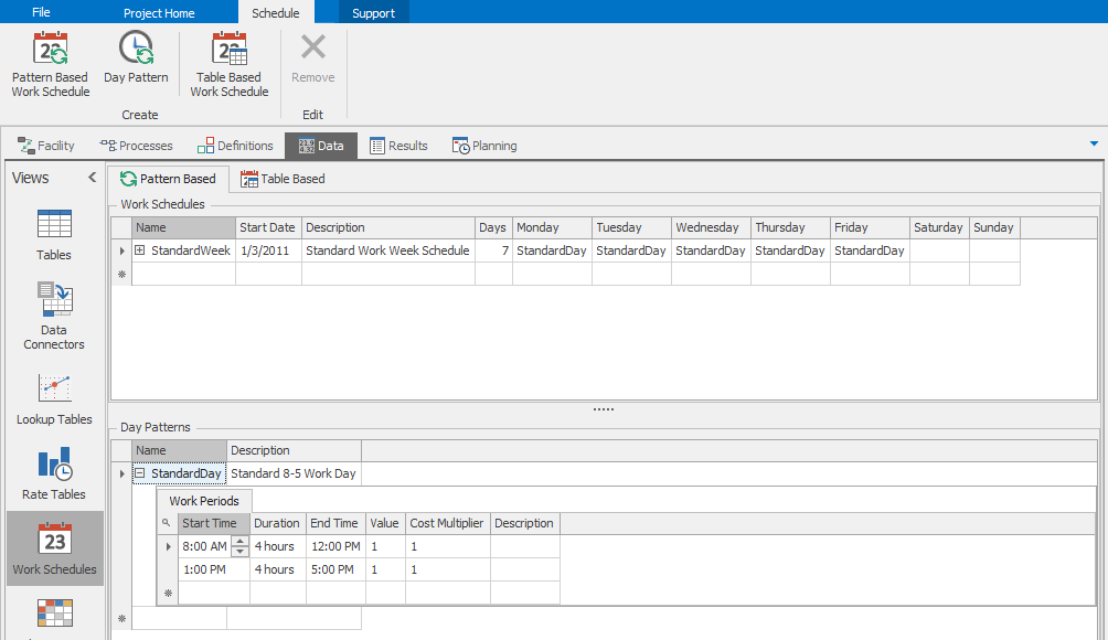
Figure 7.19: Sample pattern-based work schedule.
Simio also includes a sample work schedule named Standard Week, illustrated at the top of Figure 7.19. A Work Schedule includes a combination of Day Patterns to make up a repeating work period. The repeating period can be between 1 and 28 days; the typical situation is a seven-day week. A work period may begin on any calendar day based on the Start Date. If all of your work schedules are seven days long and start on the same day of the week (e.g., they may all start on Monday), then the column labels will be the actual days of the week. If you have schedules that start on different days of the week (e.g., one starts on Monday and another starts on Sunday), or you have any schedules that are not seven days, the column labels will simply be Day 1, Day 2, …, Day \(n\). In this case, the days that do not apply to a given schedule will be grayed out to prevent data entry.
The third component of a schedule is an Exception. An Exception overrides the repeating base schedule for the duration of the exception. Exceptions may be used to define overtime, planned maintenance, vacation periods, etc. Exceptions may be accessed by clicking the + to the left of the work-schedule name. There are two types of exceptions. The first, a Work Day Exception, indicates that on a particular day you’ll use a work pattern that differs from the normal work pattern. For example, you might define a Day Pattern called AugustFridays indicating an early quit time, then specify for all Fridays in August that you use that work pattern. The other type of exception is a Work Period Exception. This indicates that for a specific date and time range, the schedule will operate at the indicated Value, regardless of what’s specified in the schedule; this is often used for shut-down periods and extended work periods.
If you have a lot of schedules, the pattern-based schedules can be tedious to enter, especially if the data already exists in a database. For that situation, Simio offers Table-Based Work Schedules. These schedules require the same information as a day pattern, but are specified by simply describing in which table to look and which columns contain the information for the start time, end time, value, and cost multiplier of each period (see Figure 7.20).
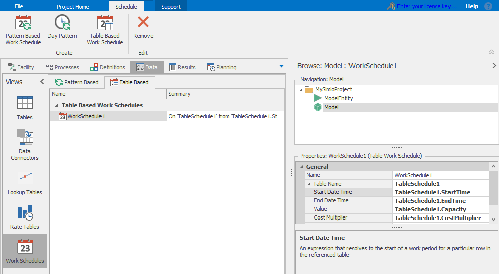
Figure 7.20: Sample table-based work schedule.
Search for “Schedule” in the Simio Help or Simio Reference Guide for a full explanation of how to configure and use calendar work schedules.
7.2.2 Manual Schedules
While calendar schedules are convenient for some applications, in other applications you might want the additional control, or perhaps simplicity, provided by a manual schedule. At the most basic level, manual schedules can be quite simple. You simply assign the capacity to the desired value, delay by the time it will remain at that value, and repeat as needed. For example, to create a repeating eight-hour-per-day schedule for a Server named Server1:
Double click on the
InitializedAdd-on Process Trigger. This process will be automatically executed once when the Server object is initialized.Add an Assign step, a Delay step, another Assign step, and another Delay step. Use these to set Server1.CurrentCapacity to
1, Delay by8 hours, set Server1.CurrentCapacity to0, and Delay by16 hours.Drag the End connector back to the first Assign step as illustrated in Figure 7.21. This will cause the four steps to keep repeating indefinitely.
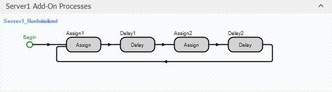
Figure 7.21: Manually created schedule of 8 working hours per day.
Manual schedules also provide great flexibility. You can add as much detail as you want, as well as add transition logic. For example, you might implement logic that says at lunch, the resource would just immediately stop working or Suspend any work in progress and then at the end of lunch he would Resume that work where he left off. But you could also implement logic so that 30 minutes before the end of the shift, he’d stop accepting new work (to allow time for cleanup), but if work was still in progress at the end of the shift he’d continue working until it was complete. This was just one example, but with the full power of processes available, sophisticated schedule behavior can be modeled. You can make objects as intelligent as your model requires.
7.3 Rate Tables and Model 7-4
A Rate Table is very different from the previous tables we’ve discussed — it’s not general-purpose and doesn’t allow adding your own columns. Rather, it’s dedicated to a single purpose: specifying time-varying entity arrival rates by time period. While our applications so far have primarily involved constant arrival rates for the duration of a run, many commonplace applications have arrival rates that vary over time, especially service applications. For example, customers come into a bank more frequently during some periods than other periods. Callers call for support more at certain times of the day than at others.
For previous models we’ve often assumed a stationary Poisson process, in which independent arrivals occurred one at a time according to an exponential interarrival-time probability distribution with a fixed mean. To implement arrival rates that vary over time, we need a nonstationary Poisson process. See Section 6.2.3 for a general discussion of this kind of arrival process, and the need to include arrival-rate “peaks” and “valleys” in the model if they’re present in reality, for the sake of model validity.
While you might think that you could stick with an exponential interarrival-time distribution and simply specify the mean interarrival time as a state and vary the value of that state at discrete points in time, you would be incorrect. Following that approach yields incorrect results because it doesn’t properly account for the transition from one period to the next. Use of the Rate Table provides the correct time-varying arrival-rate capability that we need.
A Rate Table is used by the Source object to generate entities according to a nonstationary Poisson process with a time-varying arrival rate. You can specify the number of intervals as well as the interval time duration. The Rate Table consists of a set of equal-duration time intervals and specification of the mean arrival rate during each interval, which is assumed to stay constant during an interval but can change at the start of the next interval. The rate for each interval is expressed in Arrivals per Hour, regardless of the time units specified for the intervals of the Rate Table (e.g., even if you specify a time interval of ten minutes, the arrival rate for each of those ten-minute intervals must still be expressed as a rate per hour). The Rate Table will automatically repeat from the beginning once it reaches the end of the last time interval. Though it might seem quite limiting to have to model an arrival-rate function as piecewise-constant in this way, this actually has been shown to be a very good approximation of the true underlying rate function in reality; see(Leemis 1991).
To use a Rate Table with the standard Source object, set the Arrival Mode property in the Source to Time Varying Arrival Rate and then select the appropriate Rate Table for the Rate Table property.
Let’s illustrate this concept by enhancing our ED Model 7-2 with more accurate arrivals. While our initial model approximated our arrivals with a fixed mean interarrival time of 4 minutes, we know that the arrival rate varies over the day. More specifically, we have data on the average number of arrivals for each four-hour period of the day as shown in Table 7.5.
| Time Period | Average Number of Patients Arriving in Time Period |
|---|---|
| 0:00 to 4:00 | 49 |
| 4:00 to 8:00 | 31 |
| 8:00 to 12:00 | 38 |
| 12:00 to 16:00 | 36 |
| 16:00 to 20:00 | 60 |
| 20:00 to 24:00 | 70 |
So let’s add that to our model.
Start with Model 7-2. Select the
Datawindow and theRate Tablespanel.Click the
Rate Tableribbon button to add a new Rate Table. Change the name toED_Arrivals.While we could leave the default and specify the arrival rate for 24 one-hour periods, we have information for only six four-hour periods. So we’ll set the table property Interval Size to
4 Hoursand set the Number of Intervals to6.Our information is specified as the average number of patients arriving in a four-hour period, but we need to specify our rates as patients per hour. Divide each rate in Table 7.5 by 4 and then enter it into the Simio Rate Table. When you’re done it should look like Figure 7.22.
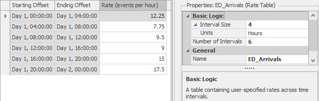
Figure 7.22: Rate Table showing time-varying patient arrival rates.
- We have one more task. We need to go back to the Facility Window and change our Source to use this Rate Table. For the Arrival Mode property, select
Time Varying Arrival Rate. For the Rate Table property, selectED_Arrivalsas shown in Figure 7.23.
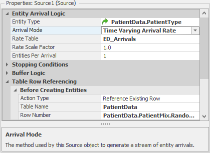
Figure 7.23: Source using Time Varying Arrival Rate.
Now if you run the model you’ll see different results, not only because of the overall lower patient load, but also because the model now has to deal with peak arrival periods with a high incoming-patient load.
Although we did not use it in this model, the Source object also includes a Rate Scale Factor property that can easily be used to modify the values within the table by a given factor instead of changing the values separately. For example, to increase the Rate Table values by 50%, simply specify the Rate Scale Factor within the Source to 1.5. This makes it easy to experiment with changing service loads (e.g., how will the system respond if the average patient load increases by 50%?).
7.4 Lookup Tables and Model 7-5
Sometimes you need a value (e.g., processing time) that depends on some other value (e.g., number of completed cycles). Sometimes a simple formula will do (e.g., Server1.CycleCount * 3.5 or Math.Sqrt( Server1.CycleCount )) or you can do a direct table lookup (e.g., MyTable[ Server1.CycleCount ].ProcessTime). Other applications can benefit from a non-linear lookup table. A Lookup Table is a special-purpose type of table designed to meet this need. It supplies an \(f(x)\) capability where \(x\) can be time, count, or any other independent variable or expression. One common application of this is modeling a learning curve where the time to perform a task might depend on the experience level of the person, measured in time or occurrences of the activity. Another application might be to determine something like processing time or battery discharge rate based on a part size or weight.
You create lookup tables in the Data Window on the Lookup Tables panel. You add a table by clicking Lookup Table on the ribbon. The table contains columns for the \(x\) (independent) value and the \(f(x)\) (dependent) value. You can use a lookup table in an expression by specifying it in the general format TableName[X_Expression], where TableName is the name of the lookup table, and X_Expression (specified as any valid expression) is the independent index value. For example, ProcessingTime[Server1.CycleCount] returns the value from the lookup table named ProcessingTime based on the current value of the Server1.CycleCount state. The lookup table value returns the defined value or a linear interpolation between the defined values. If the index is out of the defined range then the closest endpoint (first/last) point in the range is returned.
Let’s enhance Model 7-4 to add a lookup table for adjusting the Registration Time. Let’s assume that the registration process uses a computer system that’s faster in the early morning and evening, but slower during mid-day, as shown in Figure 7.24.
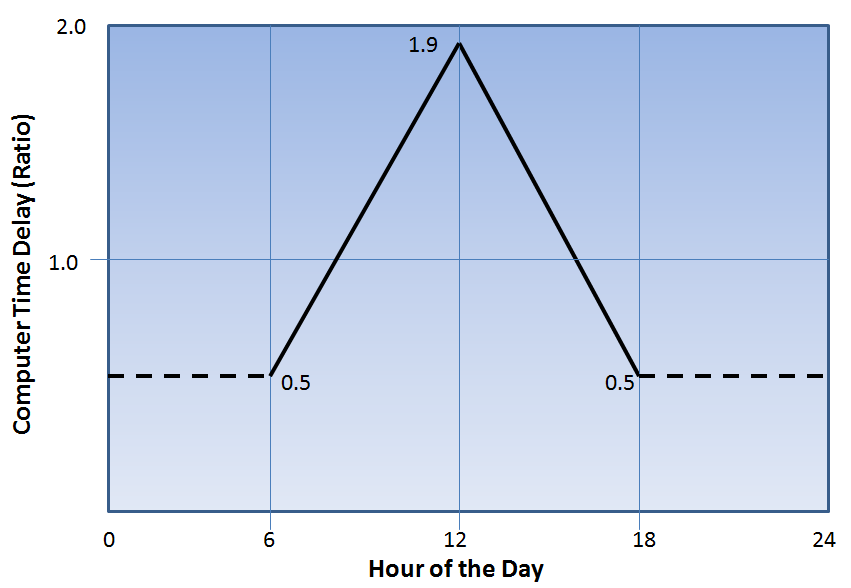
Figure 7.24: Computer responsiveness (speed factor) by time of day.
We’ll use a lookup table to apply an adjustment factor to the processing time to account for that computer speed.
Start with Model 7-4. Select the
Datawindow and theLookup Tablespanel.Click
Lookup Tableto add a new lookup table. Change the name toComputerAdjustment.Add the data to represent what’s in Figure 7.24. You have only three data points: At time
6the value0.5, at time12the value1.9, and at time18the value0.5. Any times before 6 or after 18 will return the first or last value (in this case, both 0.5). A time of exactly 12 will produce the exact value of 1.9. Any other times will interpolate linearly between the specified values. For example at time 8, it’s 1/3 of the way between the two \(x\) values, so it will return a value 1/3 of the way between the \(f(x)\) values: 0.5 + 0.466 = 0.966.The last thing we need to do is go back to the Registration server in the Facility window and amend our Processing Time. Start by right clicking on the
Process Timeproperty and selectingReset. We want to multiply the processing time specified in the Treatments table by the computer responsiveness factor we can get from our new lookup table. We need to pass the lookup table a value that represents the elapsed hours into the current day. We can take advantage of Simio’s built-in set of DateTime functions to use the one which returns the hour of the day. So the entire expression for the Registration Process Time property isTreatments.ServiceTime * ComputerAdjustment[DateTime.Hour(TimeNow)]
Now our revised model will shorten the registration time during the night and lengthen it during the day to account for the computer’s mid-day slow response.
7.5 Lists and Changeovers
In Section 5.4 we introduced the concept of Lists. Lists are used to define a collection of strings, objects, nodes, or transporters. Lists are also used to define the possible changeover states for a changeover matrix (e.g., color, size, etc.), or to provide a list from which a selection is to be made (e.g., a resource to seize, transporter to select, etc.). A List is added to a model from the Lists panel within the Definitions window.
The members of a list have a numeric index value that begins with 0. A List value may be referenced in an expression using the format List.ListName.Value. For example, if we have a list named Color with members Red, Green, Blue, and Yellow, then List.Color.Yellow returns a value of 3. If we have a ListProperty (i.e. a property whose possible values are list members) named BikeColor we can test conditions like BikeColor == List.Color.Yellow.
We will discuss the application of other types of Lists in Section 8.2.7.3, but for now we will just consider a String List. As you can easily infer from the name, a String List is simply a list of Strings. These are used primarily when you want to identify an item with a human readable string rather than a numeric equivalent.
String lists are easily constructed. In the Lists panel within the Definitions window, simply click on the String button to create a new String List. In the lower section of the window type in the strings for each item in the list like the example above as shown in Figure 7.25.
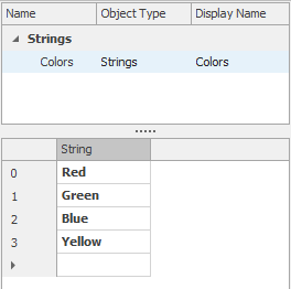
Figure 7.25: Example of a string list for colors.
A changeover is the general term used to describe the transition required between different entity types. In manufacturing this transition could be from one part size to another (e.g., large to small) or some other characteristic like color. Changeovers are not as commonly used in service applications, but are still occasionally encountered. For example the cleanup time or transition between two Routine patients might be significantly less than that of a Serious or Urgent patient. Changeovers are built into the Task Sequences section of Server (discussed in Section 10.4) and related objects, but can also be added to other objects using add-on processes.
There are three types of changeovers: Specific, Change-Dependent, and Sequence-Dependent. The simplest changeover is Specific, where every entity uses the same expression. It could be a simple constant-value expression (e.g., 5.2 minutes) or a more complex expression perhaps involving an entity state or table lookup (e.g., Entity.MySetuptime or MyDataTable.ThisSetupTime). The other types of changeovers require that you keep track of some information about the last entity that was processed and compare that to the entity about to be processed. In Change-Dependent we don’t care what the exact values are, just if it has changed. For example, if the color as changed we need one changeover time, and if it has not changed we need another (possibly 0.0) changeover time. In Sequence-Dependent, we’re usually tracking change between a discrete set of values. That set of values is typically defined in a Simio List (e.g., Small, Medium, and Large). Each unique combination of these from and to values might have a unique changeover time. This requires another Data Window feature called a Changeover Matrix.
A Changeover Matrix has a matrix based on a list. In many cases the list will be a list of Strings that identify the characteristic by name (e.g., a List named Colors that contains items Red, Green, Blue, and Yellow). The entity will typically have a property or state (e.g., Color) that contains a value from the list. The Changeover Matrix starts with the values in the specified list and displays it as a from/to matrix. In each cell you’d place the corresponding changeover time required to change from an entity with the From value to an entity with the To value. When the changeover Matrix is applied, the row is selected based on this value for the previous entity, and the column is selected based on this value for the current entity.
You can define a changeover matrix on the Changeover Matrices panel of the Data window. Click the Changeover Matrix button on the ribbon to add a new changeover. Then specify the name of your previously created list in the List Name property. At this point the lower window will expand to show a matrix of all the members of your list. You can then change the value at each intersection to indicate the transition time between pairs. In Figure 7.26 it shows a 10 minute delay to change to Yellow, but only a 2 minute delay to change to any other color, and no delay if the color remains the same.
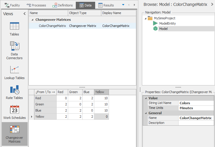
Figure 7.26: Example of a changeover matrix based on color.
7.6 State Arrays
In Section 5.1.2.2 we introduced states, but deferred two important topics — arrays and initialization. A state array is simply a set of related states. By default a state is scalar — it has a Dimension (or set size) of 0.
A state can be made into an array by changing the value of the Dimension property. If the Dimension property is set to Vector (or a 1 is typed into the Dimension property), the State is one-dimensional and the Rows property will determine the number of rows in the array. If the Dimension property is set to Matrix (or a 2 is typed into the Dimension property), the Rows and Columns properties will determine the number of rows and columns in the matrix. If you’d like an array larger than 2 dimensions, Simio supports up to 10 dimensions — just type an integer up to 10 into the Dimension property.
Referencing state arrays uses the general form StateName[row], StateName[row, column], or StateName[row, column, dimension 3, ..., dimension 10]. For example, to reference row 7, column 5 of a state array named Weight, you’d use Weight[7,5]. Note that all state-array indexing is based at 1 (e.g., a vector with 5 array elements is addressed using 1-5, not 0-4).
Each state has an Initial Value property that can be used to initialize all items in the array to the same value. If you want to initialize the items to unique values you can do so using the Assign step in a process — possibly the OnInitialized process for an object. Alternatively, you could initialize a state or state array using a Read step to read the initial values from an external data source.
An even-easier approach takes care of dimensioning and initialization all at once — set the Dimension property of the state to [Table]. First, this will automatically dimension the state array based on the table contents. Each row in the table will generate a row in the array, and each numeric column in the table (e.g., an integer, expression, date-time, …, but not an Element, Object Reference, …) will generate a column in the state array. Second, during initialization it will evaluate each numeric field and copy the values into the appropriate state-array item. If you combine this with the capability to Bind a table to an external file, this provides the capability to easily create and populate an array that exactly matches an external data source.
7.7 Data Driven Models
Often we wish to create models with reusable components. For example, perhaps we have a complex workstation – once we have that workstation built and debugged we might want to reuse that for similar workstations in the same or other facilities. While the use of objects can be an important part of the solution, the use of objects that get their data from data tables permits even more flexibility.
Sometimes we want to extend that concept to make the entire model reusable. This is useful, for example when you have a number of similar systems (e.g., ports, factories, or hospitals) where each facility is similar to the others but differs primarily in configuration and operational data.
Fortunately we can accomplish both goals by using generic components or building generic models. Data driven or sometimes Macro modeling is the concept of creating generic models with much of the key data “passed in” rather than explicitly specified in the objects. Each visiting entity could supply its own data to the object to determine how it is processed. The object would be configured to process the entity by following instructions from the entity or elsewhere in associated data tables. This concept then allows the objects to be relatively simple and of relatively few types, since the customization is primarily the responsibility of the entity and configuration data more than that of the object. The data is abstracted from the objects – instead of the data being spread across many objects, it can be consolidated in one place. This is often referred to as a data driven model.
Simio provides several features to support data-driven modeling and we have already covered some of them. Late in Section 5.1.2 we discussed using Referenced Properties as Controls to make key parameters easy to find and change. Using a control is a simple way of making a model somewhat data driven because key data can be supplied via the control values in model properties or an experiment.
In Model 7-2 we implemented a slightly more comprehensive form of data driven modeling by supplying patient type, patient mix, processing location, and processing times in a table to avoid embedding that data directly into the model objects. So instead of specific actions, our model objects essentially said, “Create the patient types specified in the table, in the percentage specified in the table, move to the location specified in the table, then process for the time specified in the table.” So now, someone with little model knowledge can experiment with our model by simply changing the data tables.
The object reference and element reference states and properties let us take this concept even further. Recall that, as the name implies, object references specify an object or a list of objects. This would allow us to extend our previous model for example, to specify the list of employees or equipment (resources) that are needed to treat or escort each type of patient. Likewise element references specify an element such as a material or statistic. This would allow you to specify any extra materials (like a surgery pack) needed by a patient or perhaps the specific statistic where a patient’s data should be recorded.
7.7.1 Tables and Repeat Groups
A discussion of data-driven modeling would be incomplete without discussing Simio’s unique relationship between tables and Repeat Groups. Recall that a repeat group is a set of properties that can be repeated across a number of rows. One example we have seen is the Assignments that are available on most objects (e.g., a Source). If you think a repeat group sounds a lot like a table, you are right. One way of looking at a repeat group is to think of it as a table that is embedded in an object. In fact, Simio allows you to freely convert between tables and repeat groups.
Let’s illustrate with a simple example. Assume that we have a list of state assignments we want to make, but we want to specify that data in a table rather than in an object.
Start with a new model and add a single Source.
Go to the
DataTab where we would add a new table, but instead of clicking the Add Data Table button, click on the pull down arrow of that button. This allows you to create a new data table matching any schema (or table layout) defined in your model.For this model, you want to scroll down and select the
Sourceschema. A table, like the one in Figure 7.27, will show up.
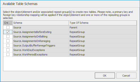
Figure 7.27: Data schemas defined by Source object.
Select the box in the Create column corresponding to the
Source.AssignmentsBeforeExitingschema. This will create a new table with the first column expecting a State Variable and the second column expecting an expression for the value that you want to assign to that state. Name your new tableStartingAssignments.Let’s add three rows to the table as illustrated in Figure 7.28. In the first row we will increment the model’s Cost state by
100. In the second and third rows we will assign the model entity’s Priority and Picture states to3and1respectively.
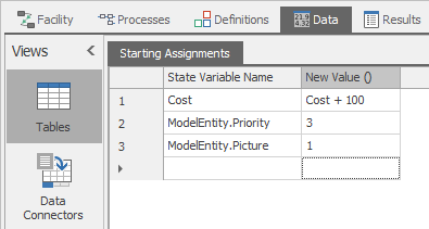
Figure 7.28: Sample assignments defined in a table.
- Now that we have created and populated our table, we can use it by using the same Referenced Property feature we have previously used. Go to the Source object in the Facility view and right click on the property name of the
Before Exitingproperty under State Assignments. Instead of creating a new referenced property, you will see that we can select the table we just defined – it’s already on the list (Figure 7.29. After you select it, you will see the same green arrow we have seen with referenced properties and the context is the same – indicating the place to go to get the data, this time referring to a collection of data in one or more rows of a table.
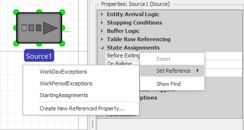
Figure 7.29: Referenced property specifies table data for a repeat group.
While this was just a very simple use of a table to populate a repeat group, when this technique is combined with the use of relational data tables it opens up many new possibilities of linking objects and data tables together to more completely implement data-driven modeling. In Sections 12.11 and 12.12 we will build simple data-driven scheduling models using a model-first approach and then a data-first approach.
The primary purpose of macro modeling is to create a somewhat abstract object that can handle many different things – like an object that represents a number of similar servers. The primary purpose of data driven modeling is to abstract the data so it can be maintained in a single place to make experimentation and model maintenance easier. While macro modeling and data driven modeling have different goals, they share the same techniques of creating somewhat generic objects that get their data from outside the object rather than directly in object properties. And these techniques often allow your model to be simpler to understand, use, and maintain.
7.8 Data Generated Models
We’ll close this chapter with one final data concept — generating models from existing data. Data Generated Models or sometimes Data First is the concept of creating generic models with much of the data for the model constructs themselves imported from external files. This can be a real “game changer” in opening ways that simulation can be of value. The ability to build models faster with less modeling expertise is obviously compelling. Beyond that, the Digital Twin discussed in Section 12.5.1 involves large models that are frequently changing. Data generated models provide an effective solution with options to bind to any data source using direct database binding, spreadsheet and CSV binding, and XML transformation. The model can then be successfully deployed in the role as Digital Twin to support design, planning, and scheduling.
There are many different situations where building models directly from existing data is desirable. Organizations often like to build business process models in flow charting tools like Microsoft Visio. While standard Visio stencils typically don’t contain all the data necessary to make a complete simulation model, custom or extended stencils may have enough information to do so. Importing that model (not only the data, but the model constructs themselves) into a full simulation package allows additional stochastic, time-based analysis and the possibility of extending the flow chart model with additional simulation constructs. This is a simple domain-neutral application of generating a model from existing data. You can find an example in the Simio Shared Items folder that facilitates this approach.
There are several international data standards which many organizations use to represent their data. B2MML, short for Business to Manufacturing Markup Language, is one popular data standard.
“B2MML is an XML implementation of the ANSI/ISA-95 family of standards (ISA-95), known internationally as IEC/ISO 62264. B2MML consists of a set of XML schemas […] that implement the data models in the ISA-95 standard. Companies […] may use B2MML to integrate business systems such as ERP and supply chain management systems with manufacturing systems such as control systems and manufacturing execution systems.” (ISA-95.com 2016)
While you could model your data configuration, imports, and exports as discussed in Section 7.1, Simio has provided an alternative. First, recognize that when companies follow a data standard such as B2MML, it generally goes beyond simply one table – it is extended to a set of data and modeling techniques. To support that Simio has implemented a feature called Templates. Somewhat similar to templates in other products (for example a resume template in Word) a Simio template consists of a skeleton for implementing a project in a standard way, potentially including data table schemas, custom objects, and relationships between those objects and the data tables.
You can apply a template when you first start a new project. Select File \(\rightarrow\) New From Template and you will see the options illustrated in
Figure 7.30. Two ISA95 (B2MML) data schemas are provided based on whether your data is order-based or product-based. When you start a new project with either of these schemas, you will find that your model has been preconfigured with relational data table schemas (but no data) and custom objects, and those custom objects are already connected to configure themselves directly from the data tables. Existing data following the ISA95 standard should be importable into these tables. Note: Since ISA95 is a guideline, company implementations are often slightly different than the standard, but you can customize the Simio data tables or create a transformation to convert between them. MESA (Manufacturing Enterprise Solutions Association)(International 2018) is one good source of information on the B2MML standard. In Section 12.12 we will build a model based on B2MML data files.
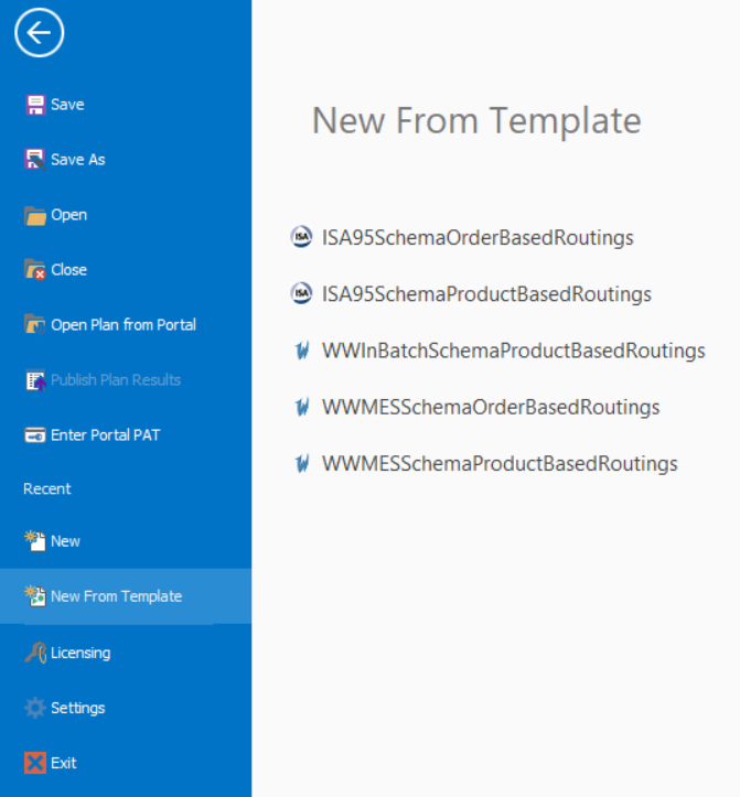
Figure 7.30: Templates available when beginning a new project.
Manufacturing Execution Systems (MES) are software-based systems that primarily track and control production, concentrating mostly on the physical operation. To work effectively they have to be based on a “model”. Similar to the ISA95 examples above, Simio can extract data directly from a MES and build and configure a Simio model from that data. In Figure 7.30 the bottom three templates are designed to create data tables with schemas to support data from Wonderware (a popular MES product from AVEVA). A similar process can be used to extract ERP data directly from a product like SAP. In fact, if you are wondering if you can create your own templates, you can! You can create your own data schemas (without data) and matching objects and save it in the Templates folder and it will appear on the list of templates to choose from.
Simio includes a feature that allows you to Auto-Create model components and their properties based on the contents of imported tables and relational tables. Refer to the Simio help topic Table-Based Elements (Auto-Create) for detailed instructions. In fact, this capability is already built into the template described above. When you import a Resources table, for example, you will see the resources automatically populated in the Facility Window.
In a small number of cases, this data-generated approach will provide a complete model that is ready to run and generate meaningful results – unfortunately this is not typical. What is much more typical, but still highly valuable, is that an approach like this applied to existing data will quickly generate a base model, which in turn, can provide the basis for incremental improvements producing meaningful results along the way. If you later decide that you want complete model generation from the data files, in some cases you can enhance existing data sources to add the missing data.
7.9 Summary
Importing, storing, and accessing data is a very important part of most models. We’ve discussed several different types of data and several ways to store data in Simio. The table constructs, and particularly the relational tables, provide extremely flexible ways of handling data and a way to abstract the data from the model objects for easier model use and maintenance. Because models are so data-intensive, it is worth exploring the options to import data and even import entire models whenever possible.
7.10 Problems
In Model 7-1 we specified priority of each entity type in the data table, but we haven’t yet used it in the model. Implement that priority so that more serious patients are treated before less serious patients. Before running, what behavior do you expect? Run to determine and report the change in time in system for each entity type.
Adjust the Server capacity of the original example Model 7-1 to 4. Create an experiment containing responses for Utilization (Server1.Capacity.ScheduledUtilization) and Length of Stay (Sink1.TimeInSystem.Average). Run it for 25 replications of 100 days with a 10-day warmup period. Compare patient waiting times if the Patient Mix of the modified example Model 7-1 changed seasonally so that Urgent patients increased to 10%, Severe patients to 30%, and Moderate and Routine patients decreased to 24% and 36% respectively.
In addition to the patient categories of modified example Model 7-1 from Problem 2, a small-town emergency hospital also caters to a general category of presenting patients who are called “Returns.” These are previous patients returning for dressing changes, adjustment of braces, removal of casts and stitches, and the like. Include this category into the Patient Mix of Model 7-1 such that proportions now become Returns 8%, Routine 30%, Moderate 26%, Severe 26%, and Urgent 10%. The treatment time for this category can vary anywhere from three minutes to thirty minutes. Compare the performance with that of Problem 2.
More realistically, about two thirds of the patients of Problem 3 arrive during the daytime (8:00 a.m. – 8:00 p.m.). Without changing the overall daily arrival rate, modify the model of Problem 2 to accommodate this updated arrival pattern. Compare the performance with that of Problem 3. Collect Length of Stay (LOS) for daytime separate from night time. What change would you make to minimize staffing, while keeping average LOS for both periods under 0.5 hour?
On further analysis it is found that only 10% of returning patients of Problem 3 require treatment times between twenty and thirty minutes; the balance require between 3 and 20 minutes. What is the new LOS? Offer suggestions to management as to how to improve staff efficiency while keeping the LOS under the target of 0.5 hour.
Routine and Return patients have a somewhat low tolerance (30 to 90 minutes) for waiting for treatment and will sometimes leave without being seen (LWBS). The other categories of “really sick” patients will always wait until they are treated. Modify the model of Problem 3 so that any patient who waits more than his or her tolerance will exit the system. Report on the waiting times and the percentage of total patients who left without treatment.
A small free clinic has a single doctor who sees patients between 8:00 a.m. and noon. She spends 6 to 14 minutes (an average of 10) with each patient and so can theoretically see 6 patients per hour or a total of 24 each day. Staff is currently scheduling patient arrivals every 10 minutes, but have found that patients arrive as much as 15 minutes early or 30 minutes late, thus causing disruption to other patients. Worse, about 10 percent of patients never show up at all causing the doctor’s time to be wasted and wasting an appointment that could have been used by other sick patients. Staff would like to evaluate alternative scheduling strategies such as scheduling 2-3 arrivals every 20 minutes with the main objective of maximizing the doctors utilization (e.g., she would like to really see 24 patients each day if possible). Assume that the doctor will stay until all scheduled patients are seen, but she is very unhappy if she needs to stay past 12:30. Measure system performance mainly on the number of patients actually seen, but also consider the average patient waiting time, and how late the doctor must typically stay to see all scheduled patients.
Of great concern to emergency-department staff are those patients who on arrival are classified Severe but whose condition before receiving treatment deteriorates to Urgent, requiring immediate attention and stabilization in the Trauma Rooms. If such deterioration is noticed during the examination stage in 10% of the Severe patients, adjust Model 7-2 to reflect this and compare the impact on waiting times and throughput. What assumptions have you made about “immediate attention?”
Emergency-department staff work 8.5 hour shifts according to an “ideal” schedule that includes a one-hour meal break each shift — preferably around mid-shift. During meal breaks, services in each section are maintained. One of “Registration” staff members will cover for the “Sign In” officer during her meal break. The minimum staffing capacity of each area is given in Table 7.6. When a new shift arrives there is a 30 minute “briefing period” during which the two shifts team together to share information and handover. Develop a defensible staffing schedule and update example Model 7-2. Re-estimate staff utilization. What assumptions do you make concerning “handover time?”
| Service Area | Minimum Capacity |
|---|---|
| Sign-In | 1 |
| Registration | 2 |
| Examination | 4 |
| Treatment Rooms | 4 |
| Trauma Rooms | 1 |
Clearly, during emergencies staff in the Trauma Rooms continue working with patients and forgo breaks — “grabbing a bite” when they can. Update Problem 9 to reflect this. Estimate the “real shift working time.”
Your task is to design and build a Simio model of a gem processing system. In our system, stones arrive from a mine and the “gem processing” consists of polishing, grading, and finishing steps where some stones require re-polishing and re-grading (see Figure 7.31 for a flow diagram). The facility works on a 24x7, three-shift basis and the stone arrivals (from the mine) are nonstationary. Table 7.7 gives the start and end times and stone arrival rates for the three shifts (note that we ignore breaks and meal times in this model and assume that there is no loss in productivity during shift-changes). You should assume that the arrival process is a non-stationary Poisson process (NSPP). The processing characteristics are given in Table 7.8. All processes have a single operator (\(c=1\)), but re-polishing and re-grading only work during first shift. In addition to the non-stationary arrivals and resource schedules, your model should have the following features:
Entities representing the stones should have the default green color when they enter the process. Those stones that require re-polishing should switch to red until they (eventually) get to Finishing, where they should switch back to green.
Create a status plot that displays the numbers of entities in the polishing and re-polishing queues along with the average number of stones in the system (3 separate items in the same plot) over time. Make the time range for your plot 24 hours.
Create a user-specified statistic that tracks the number of stones in the “re-” area — re-polishing and re-grading combined — over time.
Create a user-specified statistic that tracks the number of times each stone goes through the re-polishing process (including those stones that don’t go through re-polishing at all).
Create a user-specified statistic that tracks the time-in-system for those stones that require re-polishing (regardless of the number of times).
Create an experiment that includes 15 replications of length 200 days (each). The experiment should have the following experimental responses:
Average number of stones in the “re-” area;
Maximum number of stones in the “re-” area;
Average number of times stones go through re-polishing;
Average time-in-system for those stones that go through re-polishing;
Utilization of polishing.
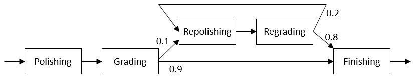
Figure 7.31: Gem processing system flow diagram for Problem 10.
| Shift | Times | Stone arrival rate |
|---|---|---|
| 1 | 7:00 a.m. - 3:00 p.m. | 30 |
| 2 | 3:00 p.m. - 11:00 p.m. | 15 |
| 3 | 11:00 p.m. - 7:00 a.m. | 5 |
| Process | Processing Times (min) | Shift 1 | Shift 2 | Shift 3 |
|---|---|---|---|---|
| Polishing | Exponential(3) | Y | Y | Y |
| Grading | Triangular(3, 3.33, 3.67) | Y | Y | Y |
| Finishing | Uniform(2, 4) | Y | Y | Y |
| Re-polishing | Exponential(7.5) | Y | N | N |
| Re-grading | Triangular(6, 7.5, 9) | Y | N | N |
References
B2MML).” Http://Www.mesa.org/En/B2MML.asp.
B2MML).” Https://Isa-95.com/B2mml/.