Chapter 4 First Model

The primary goal of this chapter is to introduce the simulation model-building process using Simio. Hand-in-hand with simulation-model building goes the statistical analysis of simulation output results, so as we build our models we’ll also exercise and analyze them to see how to make valid inferences about the system being modeled. The chapter first will build a complete Simio model and introduce the concepts of model verification, experimentation, and statistical analysis of simulation output data. Although the basic model-building and analysis processes themselves aren’t specific to Simio, we’ll focus on Simio as an implementation vehicle.

The initial model used in this chapter is very simple, and except for run length is basically the same as Model 3-4 done manually in Section 3.3.1 and Model 3-5 in a spreadsheet model in Section 3.3.2. This model’s familiarity and simplicity will allow us to focus on the process and the fundamental Simio concepts, rather than on the model. We’ll then make some easy modifications to the initial model to demonstrate additional Simio concepts. Then, in subsequent chapters we’ll successively extend the model to incorporate additional Simio features and simulation-modeling techniques to support more comprehensive systems. This is a simple single-server queueing system with arrival rate \(\lambda=48\) entities/hour and service rate \(\mu=60\) entities/hour (Figure 4.1).

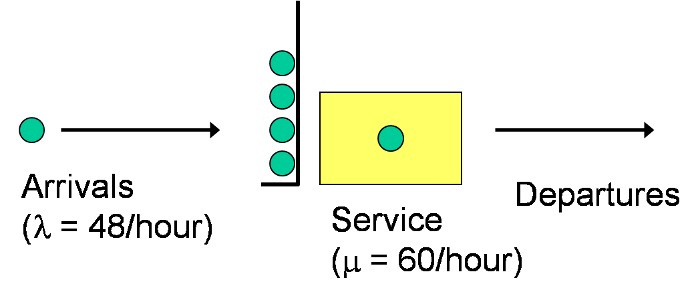
Figure 4.1: Example single-server queueing system.

This system could represent a machine in a manufacturing system, a teller at a bank, a cashier at a fast-food restaurant, or a triage nurse at an emergency room, among many other settings. For our purposes, it really doesn’t matter what is being modeled — at least for the time being. Initially, assume that the arrival process is Poisson (i.e., the interarrival times are exponentially distributed and independent of each other), the service times are exponential and independent (of each other and of the interarrival times), the queue has infinite capacity, and the queue discipline will be first-in first-out (FIFO). Our interest is in the typical queueing-related metrics such as the number of entities in the queue (both average and maximum), the time an entity spends in the queue (again, average and maximum), utilization of the server, etc. If our interest is in long-run or steady-state behavior, this system is easily analyzed using standard queueing-analysis methods (as described in Chapter 2), but our interest here is in modeling this system using Simio.

This chapter actually describes two alternative methods to model the queuing system using Simio. The first method uses the Facility Window and Simio objects from the Standard Library (Section 4.2) . The second method uses Simio Processes (Section 4.3) to construct the model at a lower level, which is sometimes needed to model things properly or in more detail. These two methods are not completely separate — the Standard Library objects are actually built using Processes. The pre-built Standard-Library objects generally provide a higher-level, more natural interface for model building, and combine animation with the basic functionality of the objects. Custom-constructed Processes provide a lower-level interface to Simio and are typically used for models requiring special functionality or faster execution. In Simio, you also have access to the Processes that comprise the Standard Library objects, but that’s a topic for a future chapter.

The chapter starts with a tour around the Simio window and user interface in Section 4.1. As mentioned above, Section 4.2 guides you through how to build a model of the system in the Facility Window using the Standard Library objects. We then experiment a little with this model, as well as introduce the important concepts of statistically independent replications, warm-up, steady-state vs. terminating simulations, and verify that our model is correct. Section 4.3 re-builds the first model with Simio Processes rather than objects. Section 4.4 adds context to the initial model and modifies the interarrival and service-time distributions. Sections 4.5 and 4.6 show how to use innovative approaches enabled by Simio for effective statistical analysis of simulation output data. Section 4.8 describes the basic Simio animation features and adds animation to the models. As your models start to get more interesting you will start finding unexpected behavior. So we will end this chapter with Section 4.9 describing the basic procedure to find and fix model problems. Though the systems being modeled in this chapter are quite simple, after going through this material you should be well on your way to understanding not only how to build models in Simio, but also how to use them.

4.1 The Basic Simio User Interface

Before we start building Simio models, we’ll take a quick tour in this section through Simio’s user interface to introduce what’s available and how to navigate to various modeling components.

When you first load Simio you’ll see either a new Simio model — the default behavior — or the most recent model that you had previously opened if you have the Load most recent project at startup checkbox checked on the File page. Figure 4.2 shows the default initial view of a new Simio model. Although you may have a natural inclination to start model building immediately, we encourage you to take time to explore the interface and the Simio-related resources provided through the Support ribbon (described below). These resources can save you an enormous amount of time.

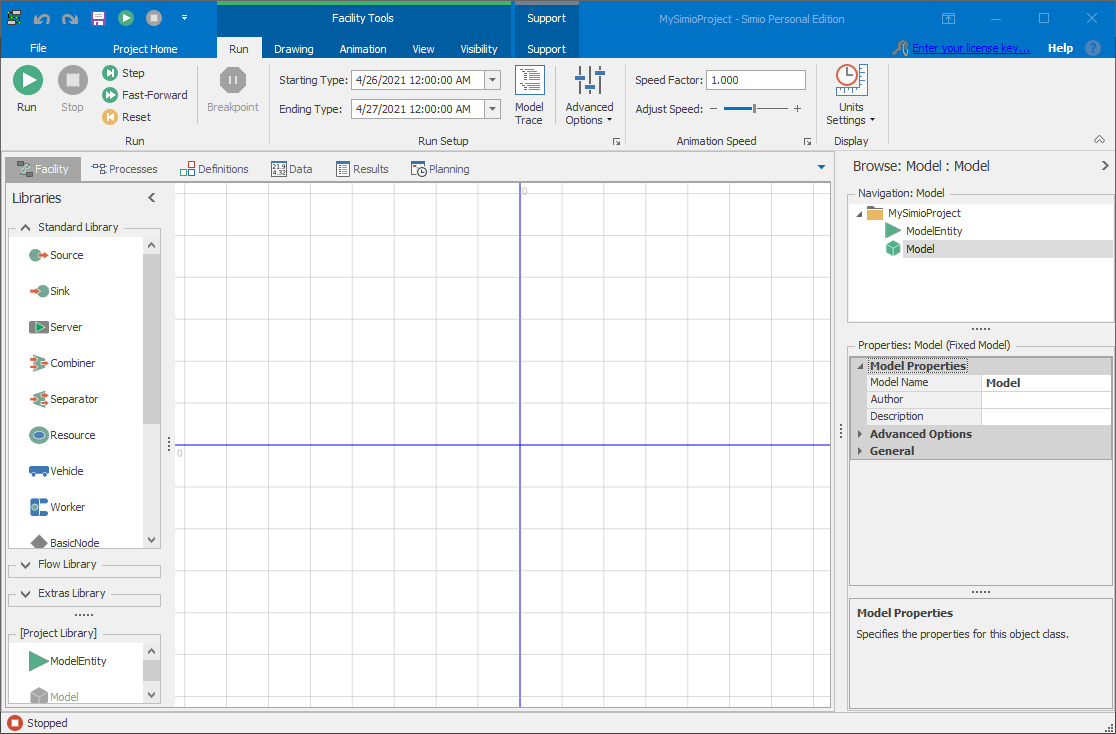
Figure 4.2: Facility window in the new model.

4.1.1 Ribbons

Ribbons are the innovative interface components first introduced with Microsoft \(^{TM}\) Office 2007 to replace the older style of menus and toolbars. Ribbons help you quickly complete tasks through a combination of intuitive organization and automatic adjustment of contents. Commands are organized into logical groups, which are collected together under tabs. Each tab relates to a type of activity, such as running a model or drawing symbols. Tabs are automatically displayed or brought to the front based on the context of what you’re doing. For example, when you’re working with a symbol, the Symbols tab becomes prominent. Note that which specific ribbons are displayed depends on where you are in the project (i.e., what items are selected in the various components of the interface).

4.1.2 Support Ribbon

The Simio Support ribbon (see Figure 4.3) includes many of the resources available to learn and get the most out of Simio, as well as how to contact the Simio people with ideas, questions, or problems. Additional information is available through the link to Simio Technical Support (http://www.simio.com/resources/technical-support/) where you will find a description of the technical-support policies and links to the Simio User Forum and other Simio-related groups. Simio version and license information is also available on the Support ribbon. This information is important whenever you contact Support.

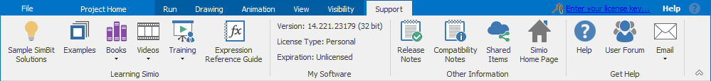
Figure 4.3: Simio Support ribbon..

Simio includes comprehensive help available at the touch of the F1 key or the ? icon in the upper right of the Simio window. If you prefer a printable version, you’ll find a link to the Simio Reference Guide (a .pdf file). The help and reference guides provide an indexed searchable resource describing basic and advanced Simio features. For additional training opportunities you’ll also find links to training videos and other on-line resources. The Support ribbon also has direct links to open example projects and SimBits (covered below), and to access Simio-related books, release and compatibility nodes, and the Simio user forum.

4.1.3 Project Model Tabs

In addition to the ribbon tabs near the top of the window, if you have a Simio project open, you’ll see a second set of tabs just below the ribbon. These are the project model tabs used to select between multiple windows that are associated with the active model or experiment. The windows that are available depend on the object class of the selected model, but generally include Facility, Processes, Definitions, Data, and Results. If you are using an RPS Simio license, you will also see the Planning tab. Each of these will be discussed in detail later, but initially you’ll spend most of your time in the Facility Window where the majority of model development, testing, and interactive runs are done.

4.1.4 Object Libraries

Simio object libraries are collections of object definitions, typically related to a common modeling domain or theme. Here we give a brief introduction to Libraries — Section \(\ref{sec-what-is-object}\) provides additional details about objects, libraries, models and the relationships between them. Libraries are shown on the left side of the Facility Window. In the standard Simio installation, the Standard Library, the Flow Library, and the Extras Libary are attached by default and the Project Library is an integral part of the project. The Standard, Flow, and Extras libraries can be opened by clicking on their respective names at the bottom of the libraries window (only one can be open at a time). The Project Library remains open and can be expanded/condensed by clicking and dragging on the .... separator. Other libraries can be added using the Load Library button on the Project Home ribbon.

The Standard Object Library on the left side of the Facility Window is a general-purpose set of objects that comes standard with Simio. Each of these objects represents a physical object, device, or item that you might find if you looked around a facility being modeled. In many cases you’ll build most of your model by dragging objects from the Standard Library and dropping them into your Facility Window. Table 4.1 lists the objects in the Simio Standard Library.

Table 4.1: Simio Standard Library objects.

Object	Description
Source	Generates entities of a specified type and arrival pattern.
Sink	Destroys entities that have completed processing in the model.
Server	Represents a capacitated process such as a machine or service operation.
Combiner	Combines multiple entities together with a parent entity (e.g., a pallet).
Separator	Splits a batched group of entities or makes copies of a single entity.
Resource	A generic object that can be seized and released by other objects.
Vehicle	A transporter that can follow a fixed route or perform on-demand pickups/dropoffs.
Worker	Models activities associated with people. Can be used as a moveable object or a transporter and can follow a shift schedule.
BasicNode	Models a simple intersection between multiple links.
TransferNode	Models a complex intersection for changing destination and travel mode.
Connector	A simple zero-time travel link between two nodes.
Path	A link over which entities may independently move at their own speeds.
TimePath	A link that has a specified travel time for all entities.
Conveyor	A link that models both accumulating and non-accu-mulating conveyor devices.

The Project Library includes the objects defined in the current project. As such, any new object definitions created in a project will appear in the Project Library for that project. Objects in the Project Library are defined/updated via the Navigation Window (described below) and they are used (placed in the Facility Window) via the Project Library. In order to simplify modeling, the Project Library is pre-populated with a ModelEntity object. The Flow Library includes a set of objects for modeling flow processing systems and the Extras Library includes a set of material handling and warehouse-related objects. Refer to the Simio Help for more information on the use of these libraries. Other domain-specific libraries are available on the Simio User Forum and can be accessed using the Shared Items button on the Support ribbon. The methods for building your own objects and libraries will be discussed in Chapter 11.

4.1.5 Properties Window

The Properties Window on the lower right side displays the properties (characteristics) of any object or item currently selected. For example, if a Server has been placed in the Facility Window, when it’s selected you’ll be able to display and change its properties in the Properties Window (see Figure 4.4. The gray bars indicate categories or groupings of similar properties. By default the most commonly changed categories are expanded so you can see all the properties. The less commonly changed categories are collapsed by default, but you can expand them by clicking on the + sign to the left. If you change a property value it will be displayed in bold and its category will be expanded to make it easy to discern changes from default values. To return a property to its default value, right click on the property name and select Reset.

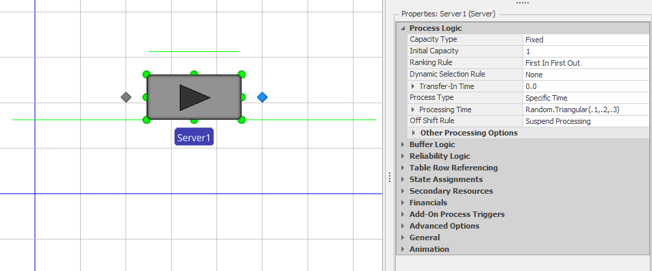
Figure 4.4: Properties for the Server object.

4.1.6 Navigation Window

A Simio project consists of one or more models or objects, as well as other components like symbols and experiments. You can navigate between the components using the Navigation Window on the upper right. Each time you select a new component you’ll see the tabs and ribbons change accordingly. For example, if you select ModelEntity in the navigation window, you’ll see a slightly different set of project model tabs available, and you might select the Definitions tab to add a state to that entity object. Then select the original Model object in the navigation window to continue editing the main model. If you get confused about what object you’re working with, look to the title bar at the top of the navigation window or the highlighted bar within the navigation window. Note that objects appearing in a library and in the Navigation Window are often confusing to new users — just remember that objects are placed from the library and are defined/edited from the Navigation Window. Additional details are provided in Section 5.1.1.1.

4.1.7 SimBits

One feature you’ll surely want to exploit is the SimBits collection. SimBits are small, well-documented models that illustrate a modeling concept or explain how to solve a common problem. The full documentation for each can be found in an accompanying automatically loaded .pdf file, as well as in the on-line help. Although they can be loaded directly from the Open menu item (replacing the currently open model), perhaps the best way to find a helpful SimBit is to look for the SimBit button on the Support ribbon. On the target page for this button you will find a categorized list of all of the SimBits with a filtering mechanism that lets you quickly find and load SimBits of interest (in this case, loading into a second copy of Simio, preserving your current workspace). SimBits are a helpful way to learn about new modeling techniques, objects, and constructs.

4.1.8 Moving/Configuring Windows and Tabs

The above discussions refer to the default window positions, but some window positions are easily changed. Many design-time and experimentation windows and tabs (for example the Process window or individual data table tabs) can be changed from their default positions by either right-clicking or dragging. While dragging, you’ll see two sets of arrows called layout targets appear: a set near the center of the window and a set near the outside of the window. For example Figure 4.5 illustrates the layout targets just after you start dragging the tab for a table. Dropping the table tab onto any of the arrows will cause the table to be displayed in a new window at that location.

Figure 4.5: Dragging a tabbed window to a new display location.

You can arrange the windows into vertical and horizontal tab groups by right clicking any tab and selecting the appropriate option. You can also drag some windows (Search, Watch, Trace, Errors, and object Consoles) outside of the Simio application, even to another monitor, to take full advantage of your screen real estate. If you ever regret your custom arrangement of the windows or you lose a window (that is, it should be displayed but you can’t find it), use the Reset button on the Project Home ribbon to restore the default window configuration.

4.2 Model 4-1: First Project Using the Standard Library Objects

In this section we’ll build the basic model described above in Simio, and also do some experimentation and analysis with it, as follows: Section 4.2.1 takes you through how to build the model in Simio, in what’s called the Facility Window using the Standard Library, run it (once), and look through the results. Next, in Section 4.2.2 we’ll use it to do some initial informal experimentation with the system to compare it to what standard queueing theory would predict. Section 4.2.3 introduces the notions of statistically replicating and analyzing the simulation output results, and how Simio helps you do that. In Section 4.2.4 we’ll talk about what might be roughly described as long-run vs. short-run simulations, and how you might need to warm up your model if you’re interested in how things behave in the long run. Section 4.2.5 revisits some of the same questions raised in Section 4.2.2, specifically trying to verify that our model is correct, but now we are armed with better tools like warm-up and statistical analysis of simulation output data. All of our discussion here is for a situation when we have only one scenario (system configuration) of interest; we’ll discuss the more common goal of comparing alternative scenarios in Sections 5.5 and 9.1.1, and will introduce some additional statistical tools in those sections for such goals.

4.2.1 Building the Model

Using Standard Library objects is the most common method for building Simio models. These pre-built objects will be sufficient for many common types of models. Figure 4.6 shows the completed model of our queueing system using Simio’s Facility Window (note that the Facility tab is highlighted in the Project Model Tabs area). We’ll describe how to construct this model step by step in the following paragraphs.

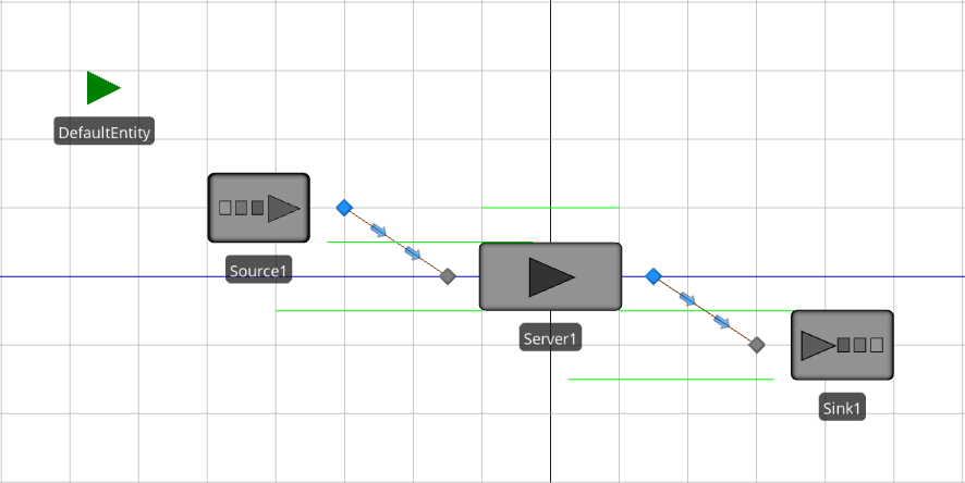
Figure 4.6: Completed Simio model (Facility Window) of the single-server queueing system — Model 4-1.

The queueing model includes entities, an entity-arrival process, a service process, and a departure process. In the Simio Facility Window, these processes can be modeled using the Source, Server, and Sink objects. To get started with the model, start the Simio application and, if necessary, create a new model by clicking on the New item in the File page (accessible from the File ribbon). Once the default new model is open, make sure that the Facility Window is open by clicking on the Facility tab, and that the Standard Library is visible by clicking on the Standard Library section heading in the Libraries bar on the left; Figure 4.2 illustrates this. First, add a ModelEntity object by clicking on the ModelEntity object in the ProjectLibrary panel, then drag and drop it onto the Facility Window (actually, we’re dragging and dropping an instance of it since the object definition stays in the ProjectLibrary panel). Next, click on the Source object in the Standard Library, then drag and drop it into the Facility Window. Similarly, click, drag, and drop an instance of each of the Server and Sink objects onto the Facility Window. The next step is to connect the Source, Server, and Sink objects in our model. For this example, we’ll use the standard Connector object, to transfer entities between nodes in zero simulation time. To use this object, click on the Connector object in the Standard Library. After selecting the Connector, the cursor changes to a set of cross hairs. With the new cursor, click on the Output Node of the Source object (on its right side) and then click on the Input Node of the Server object (on its left side). This tells Simio that entities flow (instantly, i.e., in zero simulated time) out of the Source object and into the Server object. Follow the same process to add a connector from the Output Node of the Server object to the Input Node of the Sink object. Figure 4.7 shows the model with the connector in place between the Source and Server objects.

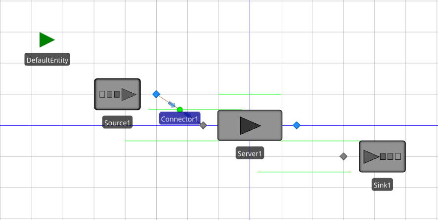
Figure 4.7: Model 4-1 with the Source and Server objects linked by a Connector object.

By the way, now would be a good time to save your model (“save early, save often,” is a good motto for every simulationist). We chose the name Model_04_01.spfx (spfx is the default file-name extension for Simio project files), following the naming convention for our example files given in Section 3.2; all our completed example files are available on the book’s website, as described in Appendix C.

Before we continue constructing our model, we need to mention that the Standard Library objects include several default queues. These queues are represented by the horizontal green lines in Figure 4.7. Simio uses queues where entities potentially wait — i.e., remain in the same logical place in the model for some period of simulated time. Note that, technically, tokens rather than entities wait in Simio queues, but we’ll discuss this issue in more detail in Chapter 5 and for now it’s easier to think of entities waiting in the queues since that is what you see in the animation. Model 4-1 includes the following queues:

• Source1 OutputBuffer.Contents — Used to store entities waiting to move out of the Source object.

• Server1 InputBuffer.Contents — Used to store entities waiting to enter the Server object.

• Server1 Processing.Contents — Used to store entities currently being processed by the Server object.

• Server1 OutputBuffer.Contents — Used to store entities waiting to exit the Server object.

• Sink1 InputBuffer.Contents — Used to store entities waiting to enter the Sink object.

In our simple single-server queueing system in Figure 4.1, we show only a single queue and this queue corresponds to the InputBuffer.Contents queue for the Server1 object. The Processing.InProcess queue for the Server1 object stores the entity that’s being processed at any point in simulated time. The other queues in the Simio model are not used in our simple model (actually, the entities simply move through these queues instantly, in zero simulated time).

Now that the basic structure of the model is complete, we’ll add the model parameters to the objects. For our simple model, we need to specify probability distributions governing the interarrival times and service times for the arriving entities. The Source object creates arriving entities according to a specified arrival process. We’d like a Poisson arrival process at rate \(\lambda = 48\) entities per hour, so we’ll specify that the entity interarrival times are exponentially distributed with a mean of 1.25 minutes (a time between entities of \(= 60/48\) corresponds to a rate of 48/hour). In the formal Simio object model, the interarrival time is a property of the Source object. Object properties are set and edited in the Properties Window — select the Source object (click on the object) and the Properties Window will be displayed on the right panel (see Figure 4.8).

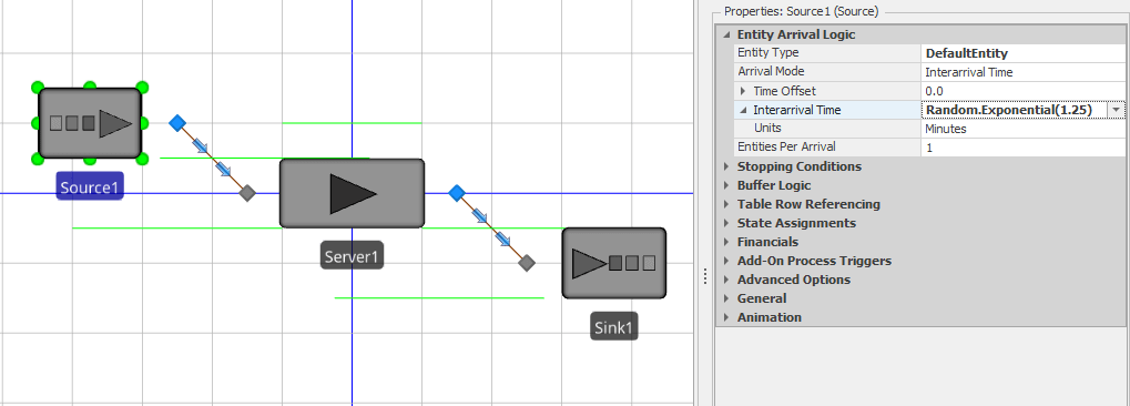
Figure 4.8: Setting the interarrival-time distribution for the Source object.

The Source object’s interarrival-time distribution is set by assigning the Interarrival Time property to Random.Exponential(1.25) and the Units property to Minutes; click on the arrow just to the left of Interarrival Time to expose the Units property and use the pull-down on the right to select Minutes. This tells Simio that each time an entity is created, it needs to sample a random value from an exponential distribution with mean \(1.25\), and to create the next entity that far into the future for an arrival rate of \(\lambda = 60 \times (1/1.25) = 48\) entities/hour, as desired. The random-variate functions available via the keyword Random are discussed further in Section 4.4. The Time Offset property (usually set to 0) determines when the initial entity is created. The other properties associated with the Arrival Logic can be left at their defaults for now. With these parameters, entities are created recursively for the duration of the simulation run.

The default object name (Source1, for the first source object), can be changed by either double-clicking on the name tag below the object with the object selected, or through the Name property in the General properties section. Or, like most items in Simio, you can rename by using the F2 key. Note that the General section also includes a Description property for the object, which can be quite useful for model documentation. You should get into the habit of including a meaningful description for each model object because whatever you enter there will be displayed in a tool tip popup note when you hover the mouse over that object.

In order to complete the queueing logic for our model, we need to set up the service process for the Server object. The Processing Time property of the Server module is used to specify the processing times for entities. This property should be set to Random.Exponential(1) with the Units property being Minutes. Make sure that you adjust the Processing Time property rather than the Process Type property (this should remain at its default value of Specific Time (the other options for processing type will be discussed in Section 10.3). The final step for our initial model is to tell Simio to run the model for 10 hours. To do this, click on the Run ribbon/tab, then in the Ending Type pull-down, select the Run Length option and enter 10 Hours. Before running our initial model, we’ll set the running speed for the model.

The Speed Factor is used to control the speed of the interactive execution of the model explicitly. Changing the Speed Factor to 50 (just type it into the Speed Factor field in the Run ribbon) will speed up the run to a speed that’s more visually appealing for this particular model. The optimal Speed Factor for an interactive run will depend on the model and object parameters and the individual preferences, as well as the speed of your computer, so you should definitely experiment with the Speed Factor for each model (technically, the Speed Factor is the amount of simulation time, in tenths of a second, between each animation frame).

At this point, we can actually run the model by clicking on the Run icon in the upper left of the ribbon. The model is now running in interactive mode. As the model runs, the simulated time is displayed in the footer section of the application, along with the percentage complete. Using the default Speed Factor, simulation time will advance fairly slowly, but this can be changed as the model runs. When the simulation time reaches 10 (the run length that we set), the model run will automatically pause.

In Interactive Mode, the model results can be viewed at any time by stopping or pausing the model and clicking on the Results tab on the tab bar. Run the model until it reaches 10 hours and view the current results. Simio provides several different ways to view the basic model results. Pivot Grid, and Reports (the top two options are on the left panel — click on the corresponding icon to switch between the views) are the most common. Figure 4.9 shows the Pivot Grid for Model 4-1 paused at time 10 hours.

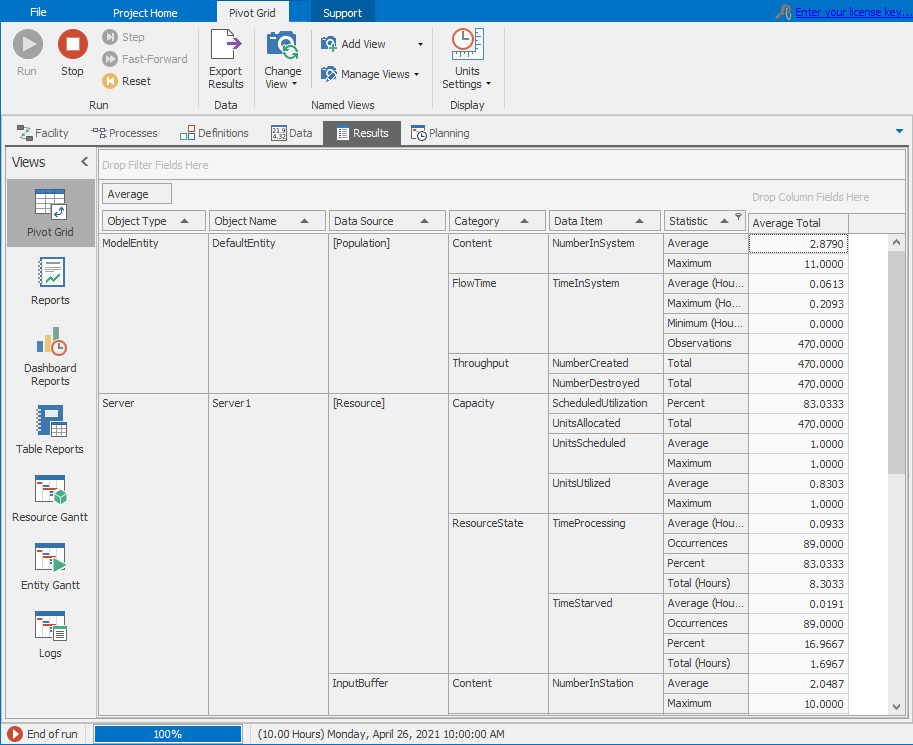
Figure 4.9: Pivot Grid report for the interactive run of Model 4-1.

Note that Simio uses an agile development process with frequent minor updates, and occasional major updates. It’s thus possible that the output values you get when you run our examples interactively may not always exactly match the output numbers we’re showing here, which we got as we wrote the book. This could, as noted at the end of Section 1.4, be due to small variations across releases in low-level behavior, such as the order in which simultaneous events are processed. Regardless of the reason for these differences, their existence just emphasizes the need to do proper statistical design and analysis of simulation experiments, and not just run it once to get “the answer,” a point that we’ll make repeatedly throughout this book. The Pivot Grid format is extremely flexible and provides a very quick method to find specific results. If you’re not accustomed to this type of report, it can look a bit overwhelming at first, but you’ll quickly learn to appreciate it as you begin to work with it. The Pivot Grid results can also be easily exported to a CSV (comma-separated values) text file, which can be imported into Excel and other applications. Each row in the default Pivot Grid includes an output value based on:

• Object Type

• Object Name

• Data Source

• Category

• Data Item

• Statistic

So, in Figure 4.9, the Average (Statistic) value for the TimeInSystem (Data Item) of the DefaultEntity (Object Name) of the ModelEntity type (Object Type) is \(0.0613\) hours (0.0613 hours \(\times\) 60 minutes/hour = 3.6780 minutes. Note that units for the Pivot Grid times, lengths, and rates can be set using the Time Units, Length Units, and Rate Units items in the Pivot Grid ribbon; if you switch to Minutes the Average TimeInSystem is 3.6753, so our hand-calculated value of 3.6780 minutes has a little round-off error in it. Further, the TimeInSystem data item belongs to the FlowTime Category and since the value is based on entities (dynamic objects), the Data Source is the set of Dynamic Objects.

If you’re looking at this on your computer (as you should be!), scrolling through the Pivot Grid reveals a lot of output performance measures even from a small model like this. For instance, just three rows below the Average TimeInSystem of 0.0613 hours, we see under the Throughput Category that a total of 470 entities were created (i.e., entered the model through the Source object), and in the next row that 470 entities were destroyed (i.e., exited the model through the Sink object). Though not always true, in this particular run of this model all of the 470 entities that arrived also exited during the 10 hours, so that at the end of the simulation there were no entities present. You can confirm this by looking at the animation when it’s paused at the 10-hour end time. (Change the run time to, say, 9 hours, and then 11 hours, to see that things don’t always end up this way, both by looking at the final animation as well as the NumberCreated and NumberDestroyed in the Throughput Category of the Pivot Grid). So in our 10-hour run, the output value of 0.0613 hours for average time in system is just the simple average of these 470 entities’ individual times in system.

While you’re playing around with the simulation run length, try changing it to 8 minutes and compare some of the Pivot Grid results with what we got from the manual simulation in Section 3.3.1 given in Figure 3.9. Now we can confess that those “magical” interarrival and service times for that manual simulation were generated in this Simio run, and we recorded them via the Model Trace capability.

The Pivot Grid supports three basic types of data manipulation:

• Grouping: Dragging column headings to different relative locations will change the grouping of the data.

• Sorting: Clicking on an individual column heading will cause the data to be sorted based on that column.

• Filtering: Hovering the mouse over the upper right corner of a column heading will expose a funnel-shaped icon. Clicking on this icon will bring up a dialog that supports data filtering. If a filter is applied to any column, the funnel icon is displayed (no mouse hover required). Filtering the data allows you quickly to view the specific data in which you’re interested regardless of the amount of data included in the output.

Pivot Grids also allow the user to store multiple views of the filtered, sorted, and grouped Pivot Grids. Views can be quite useful if you are monitoring a specific set of performance metrics. The Simio documentation section on Pivot Grids includes much more detail about how to use these specific capabilities. The Pivot Grid format is extremely useful for finding information when the output includes many rows.

The Reports format gives the interactive run results in a formatted, detailed report format, suitable for printing, exporting to other file formats, or emailing (the formatting, printing, and exporting options are available from the Print Preview tab on the ribbon). Figure 4.10 shows the Reports format with the Print Preview tab open on the ribbon. Scrolling down to the TimeInSystem - Average (Hours) heading on the left will show a Value of 0.06126, the same (up to roundoff) as we saw for this output performance measure in the Pivot Grid in Figure 4.9.

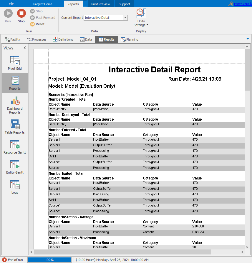
Figure 4.10: Standard report view for Model 4-1.

4.2.2 Initial Experimentation and Analysis

Now that we have our first Simio model completed, we’ll do some initial, informal experimenting and analysis with it to understand the queueing system it models. As we mentioned earlier, the long-run, steady-state performance of our system can be determined analytically using queueing analysis (see Chapter 2 for details). Note that for any but the simplest models, this type of exact analysis will not be possible (this is why we use simulation, in fact). Table 4.2 gives the steady-state queueing results and the simulation results taken from the Pivot Table in Figure 4.9.

Table 4.2: Comparison of the queueing analysis and initial model results for the first model.

Metric	Queueing	Model
Utilization (\(\rho\))	\(0.800\)	\(0.830\)
Number in system (\(L\))	\(4.000\)	\(2.879\)
Number in queue (\(L_q\))	\(3.200\)	\(2.049\)
Time in system (\(W\))	\(0.083\)	\(0.061\)
Time in queue (\(W_q\))	\(0.067\)	\(0.044\)

You’ll immediately notice that the numbers in the Queueing column are not equal to the numbers in the Model column, as we might expect. Before discussing the possible reasons for the differences, we first need to discuss one more important and sometimes-concerning issue. If you return to the Facility Window (click on the Facility tab just below the ribbon), reset the model (click on the Reset icon in the Run ribbon), re-run the model, allow it to run until it pauses at time 10 hours, and view the Pivot Grid, you’ll notice that the results are identical to those from the previous run (displayed in Figure 4.9). If you repeat the process again and again, you’ll always get the same output values. To most people new to simulation, and as mentioned in Section 3.1.3, this seems a bit odd given that we’re supposed to be using random values for the entity interarrival and service times in the model. This illustrates the following critical points about computer simulation:

1. The random numbers used are not truly random in the sense of being unpredictable, as mentioned in Section 3.1.3 and discussed in Section 6.3 — instead they are pseudo-random, which, in our context, means that the precise sequence of generated numbers is deterministic (among other things).

2. Through the random-variate-generation process discussed in Section 6.4, some simulation software can control the pseudo-random number generation and we can exploit this control to our advantage.

The concept that the “supposedly random numbers” are actually predictable can initially cause great angst for new simulationists (that’s what you’re now becoming). However, for simulation, this predictability is a good thing. Not only does it make grading simulation homework easier (important to the authors), but (more seriously) it’s also useful during model debugging. For example, when you make a change in the model that should have a predictable effect on the simulation output, it’s very convenient to be able to use the same “random” inputs for the same purposes in the simulation, so that any changes (or lack thereof) in output can be directly attributable to the model changes, rather than to different random numbers. As you get further into modeling, you’ll find yourself spending significant time debugging your models so this behavior will prove useful to you (see Section 4.9 for detailed coverage of the debugging process and Simio’s debugging tools). In addition, this predictability can be used to reduce the required simulation run time through a variety of techniques called variance reduction, which are discussed in general simulation texts (such as (Banks et al. 2005) or (Law 2015)). Simio’s default behavior is to use the same sequence of random variates (draws or observations on model-driving inputs like interarrival and service times) each time a model is run. As a result, running, resetting, and re-running a model will yield identical results unless the model is explicitly coded to behave otherwise.

Now we can return to the question of why our initial simulation results are not equal to our queueing results in Table 4.2. There are three possible explanations for this mismatch:

1. Our Simio model is wrong, i.e., we have an error somewhere in the model itself.

2. Our expectation is wrong, i.e., our assumption that the simulation results should match the queueing results is wrong.

3. Sampling error, i.e., the simulation model results match the expectation in a probabilistic sense, but we either haven’t run the model long enough, or for enough replications (separate independent runs starting from the same state but using separate random numbers), or are interpreting the results incorrectly.

In fact, if the results are not equal when comparing simulation results to our expectation, it’s always one or more of these possibilities, regardless of the model. In our case, we’ll see that our expectation is wrong, and that we have not run the model long enough. Remember, the queueing-theory results are for long-run steady-state, i.e., after the system/model has run for an essentially infinite amount of time. But we ran for only 10 hours, which for this model is evidently not sufficiently close to infinity. Nor have we made enough replications (items 2 and 3 from above). Developing expectations, comparing the expectations to the simulation-model results, and iterating until these converge is a very important component of model verification and validation (we’ll return to this topic in Section 4.2.5).

4.2.3 Replications and Statistical Analysis of Output

As just suggested, a replication is a run of the model with a fixed set of starting and ending conditions using a specific and separate, non-overlapping sequence of input random numbers and random variates (the exponentially distributed interarrival and service times in our case). For the time being, assume that the starting and ending conditions are dictated by the starting and ending simulation time (although as we’ll see later, there are other possible kinds of starting and ending conditions). So, starting our model empty and idle, and running it for 10 hours, constitutes a replication. Resetting and re-running the model constitutes running the same replication again, using the same input random numbers and thus random variates, so obviously yielding the same results (as demonstrated above). In order to run a different replication, we need a different, separate, non-overlapping set of input random numbers and random variates. Fortunately, Simio handles this process for us transparently, but we can’t run multiple replications in Interactive mode. Instead, we have to create and run a Simio Experiment.

Simio Experiments allow us to run our model for a user-specified number of replications, where Simio guarantees that the generated random variates are such that the replications are statistically independent from one another, since the underlying random numbers do not overlap from one replication to the next. This guarantee of independence is critical for the required statistical analysis we’ll do. To set up an experiment, go to the Project Home ribbon and click on the New Experiment icon. Simio will create a new experiment and switch to the Experiment Design view as shown in Figure 4.11 after we changed both Replications Required near the top, and Default Replications on the right, to 5 from their default values of 10.

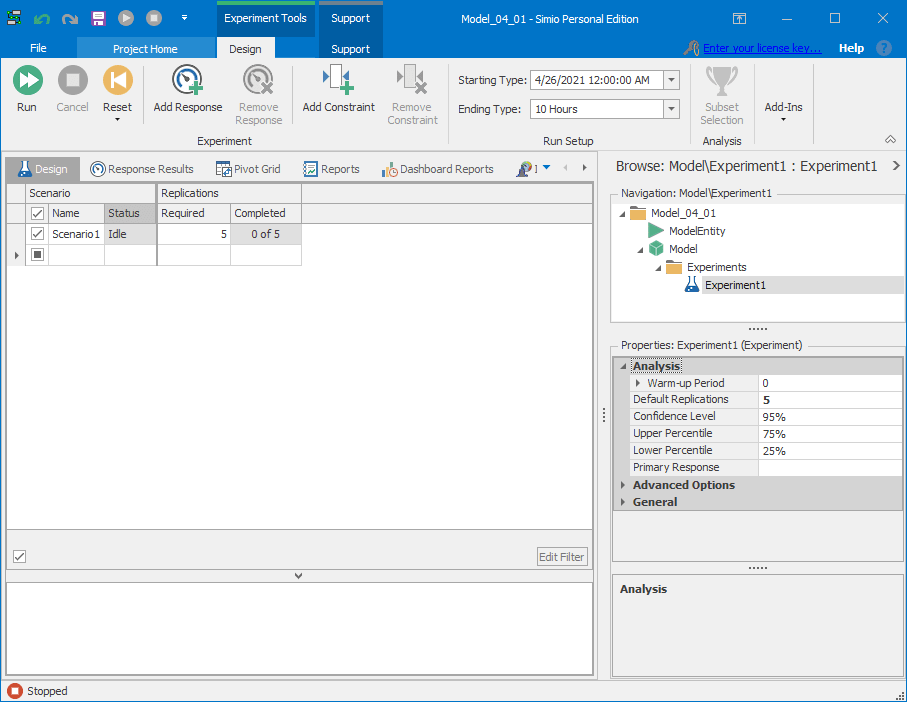
Figure 4.11: Initial experiment design for running five replications of a model.

To run the experiment, select the row corresponding to Scenario1 (the default name) and click the Run icon (the one with two white right arrows in it in the Experiment window, not the one with one right arrow in it in the Model window). After Simio runs the five replications, select the Pivot Grid report (shown in Figure 4.12).

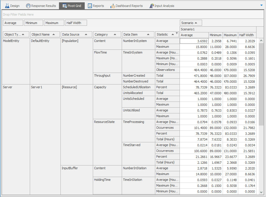
Figure 4.12: Experiment Pivot Grid for the five replications of the model.

Compared to the Pivot Grid we saw while running in Interactive Mode (Figure 4.9), we see the additional results columns for Minimum, Maximum, and Half Width (of 95% confidence intervals on the expected value, with the Confidence Level being editable in the Experiment Design Properties), reflecting the fact that we now have five independent observations of each output statistic.

To understand what these cross-replication output statistics are, focus on the entity TimeInSystem values in rows 3-5. For example:

• The 0.0762 for the Average of Average (Hours) TimeInSystem (yes, we meant to say “Average” twice there) is the average of five numbers, each of which is a within-replication average time in system (and the first of those five numbers is 0.0613 from the single-replication Pivot Grid in Figure 4.9. The 95% confidence interval \(0.0762 \pm 0.0395\), or \([0.0367, 0.1157]\) (in hours), contains, with 95% confidence , the expected within-replication average time in system, which you can think of as the result of making an infinite number of replications (not just five) of this model, each of duration 10 hours, and averaging all those within-replication average times in system. Another interpretation of what this confidence interval covers is the expected value of the probability distribution of the simulation output random variable representing the within-replication average time in system. (More discussion of output confidence intervals appears below in the discussion of Table 4.4.)

• Still in the Average (Hours) row, 0.1306 is the maximum of these five average within-replication times in system, instead of their average. In other words, across the five replications, the largest of the five Average TimeInSystem values was 0.1306, so it is the maximum average.

• Average maximum, anyone? In the next row down for Maximum (Hours), the 0.2888 on the left is the average of five numbers, each of which is the maximum individual-entity time in system within that replication. And the 95% confidence interval \(0.2888 \pm 0.1601\) is trying to cover the expected maximum time in system, i.e., the maximum time in system averaged over an infinite number of replications rather than just five.

• Maybe more meaningful as a really bad worst-case time in system, though, would be the 0.5096 hour, being the maximum of the five within-replication maximum times in system.

Table 4.3 gives the queueing metrics for each of the five replications of the model, as well a the sample mean (Avg) and sample standard deviation (StDev) across the five replications for each metric. To access these individual-replication output values, click on the Export Details icon in the Pivot Grid ribbon; click Export Summaries to get cross-replication results like means and standard deviations, as shown in the Pivot Grid itself. The exported data file is in CSV format, which can be read by a variety of applications, such as Excel. The first thing to notice in this table is that the values can vary significantly between replications (\(L\) and \(L_q\), in particular). This variation is specifically why we cannot draw inferences from the results of a single replication.

Table 4.3: Five replications of data for the first model.

Metric being estimated	1	2	3	4	5	Avg	StDev
Utilization (\(\rho\))	\(0.830\)	\(0.763\)	\(0.789\)	\(0.769\)	\(0.785\)	\(0.787\)	\(0.026\)
Number in system (\(L\))	\(2.879\)	\(2.296\)	\(3.477\)	\(2.900\)	\(6.744\)	\(3.659\)	\(1.774\)
Number in queue (\(L_q\))	\(2.049\)	\(1.532\)	\(2.688\)	\(2.131\)	\(5.959\)	\(2.872\)	\(1.774\)
Time in system (\(W\))	\(0.061\)	\(0.049\)	\(0.075\)	\(0.065\)	\(0.131\)	\(0.076\)	\(0.032\)
Time in queue (\(W_q\))	\(0.044\)	\(0.033\)	\(0.058\)	\(0.048\)	\(0.115\)	\(0.059\)	\(0.032\)

Since our model inputs (entity interarrival and service times) are random, the simulation-output performance metrics (simulation-based estimates of \(\rho\), \(L\), \(L_q\), \(W\), and \(W_q\), which we could respectively denote as \(\widehat{\rho}\), \(\widehat{L}\), \(\widehat{L_q}\), \(\widehat{W}\), and \(\widehat{W_q}\)) are random variables . The queueing analysis gives us the exact steady-state values of \(\rho\), \(L\), \(L_q\), \(W\), and \(W_q\). Based on how we run replications (the same model, but with separate independent input random variates), each replication generates one observation on each of \(\widehat{\rho}\), \(\widehat{L}\), \(\widehat{L_q}\), \(\widehat{W}\), and \(\widehat{W_q}\). In statistical terms, running \(n\) replications yields \(n\) independent, identically distributed (IID) observations of each random variable. This allows us to estimate the mean values of the random variables using the sample averages across replications. So, the values in the Average column from Table 4.3 are estimates of the corresponding random-variable expected values. What we don’t know from this table is how good our estimates are. We do know, however, that as we increase the number of replications, our estimates get better, since the sample mean is a consistent estimator (its own variance decreases with \(n\)), and from the strong law of large numbers (as \(n \rightarrow \infty\), the sample mean across replications \(\rightarrow\) the expected value of the respective random variable, with probability 1).

Table 4.4 compares the results from running five replications with those from running 50 replications. Since we ran more replications of our model, we expect the estimates to be better, but averages still don’t give us any specific information about the quality (or precision) of these estimates. What we need is an interval estimate that will give us insight about the sampling error (the averages are merely point estimates). The \(h\) columns give such an interval estimate. These columns give the half-widths of 95% confidence intervals on the means constructed from the usual normal-distribution approach (using the sample standard deviation and student’s \(t\) distribution with \(n-1\) degrees of freedom, as given in any beginning statistics text). Consider the 95% confidence intervals for \(L\) based on five and 50 replications: \[\begin{align*} 5\ \textrm{replications}: 3.659 \pm 2.203\ \textrm{or}\ [1.456, 5.862] \\ 50\ \textrm{replications}: 3.794 \pm 0.433\ \textrm{or}\ [3.361, 4.227] \end{align*}\]

Table 4.4: Comparing 5 replications (left side) with 50 replications (right side).

Metric being estimated	Avg	\(h\)	Avg	\(h\)
Utilization (\(\rho\))	\(0.787\)	\(0.033\)	\(0.789\)	\(0.014\)
Number in system (\(L\))	\(3.659\)	\(2.203\)	\(3.794\)	\(0.433\)
Number in queue (\(L_q\))	\(2.872\)	\(2.202\)	\(3.004\)	\(0.422\)
Time in system (\(W\))	\(0.076\)	\(0.040\)	\(0.078\)	\(0.008\)
Time in queue (\(W_q\))	\(0.059\)	\(0.040\)	\(0.062\)	\(0.008\)

Based on five replications, we’re 95% confident that the true mean (expected value or population mean) of \(\widehat{L}\) is between 1.456 and 5.862, while based on 50 replications, we’re 95% confident that the true mean is between 3.361 and 4.227. (Strictly speaking, the interpretation is that 95% of confidence intervals formed in this way, from replicating, will cover the unknown true mean.) So the confidence interval on the mean of an output statistic provides us a measure of the sampling error and, hence, the quality (precision) of our estimate of the true mean of the random variable. By increasing the number of replications (samples), we can make the half-width increasingly small. For example, running 250 replications results in a CI of \([3.788, 4.165]\) — clearly we’re more comfortable with our estimate of the mean based on 250 replications than we are based five replications. In cases where we make independent replications, the confidence-interval half-widths therefore give us guidance as to how many replications we should run if we’re interested in getting a precise estimate of the true mean; due to the \(\sqrt{n}\) in the denominator of the formula for the confidence-interval half width, we need to make about four times as many replications to cut the confidence interval half-width in half, compared to its current size from an initial number of replications, and about 100 times as many replications to make the interval \(1/10\) its current size. Unfortunately, there is no specific rule about “how close is close enough” — i.e., what values of \(h\) are acceptably small for a given simulation model and decision situation. This is a judgment call that must be made by the analyst or client in the context of the project. There is a clear trade-off between computer run time and reducing sampling error. As we mentioned above, we can make \(h\) increasingly small by running enough replications, but the cost is computer run time. When deciding if more replications are warranted, two issues are important:

1. What’s the cost if I make an incorrect decision due to sampling error?

2. Do I have time to run more replications?

So, the first answer as to why our simulation results shown in Table 4.2 don’t match the queueing results is that we were using the results from a singe replication of our model. This is akin to rolling a die, observing a 4 (or any other single value) and declaring that value to be the expected value over a large number of rolls. Clearly this would be a poor estimate, regardless of the individual roll. Unfortunately, using results from a single replication is quite common for new simulationists, despite the significant risk. Our general approach going forward will be to run multiple replications and to use the sample averages as estimates of the means of the output statistics, and to use the 95% confidence-interval half-widths to help determine the appropriate number of replications if we’re interested in estimating the true mean. So, instead of simply using the averages (point estimates), we’ll also use the confidence intervals (interval estimates) when analyzing results. The standard Simio Pivot Grid report for experiments (see Figure 4.12) automatically supports this approach by providing the sample average and 95% confidence-interval half-widths for all output statistics.

The second reason for the mismatch between our expectations and the model results is a bit more subtle and involves the need for a warm up period for our model. We will discuss that in the next section.

4.2.4 Steady-State vs. Terminating Simulations

Generally, when we start running a simulation model that includes queueing or queueing-network components, the model starts in a state called empty and idle, meaning that there are no entities in the system and all servers are idle. Consider our simple single-server queueing model. The first entity that arrives will never have to wait for the server. Similarly, the second arriving entity will likely spend less time in the queue (on average) than the 100th arriving entity (since the only possible entity in front of the second entity will be the first entity). Depending on the characteristics of the system being modeled (the expected server utilization, in our case), the distribution and expected value of queue times for the third, fourth, fifth, etc. entities can be significantly different from the distribution and expected value of queue times at steady state, i.e., after a long time that is sufficient for the effects of the empty-and-idle initial conditions to have effectively worn off. The time between the start of the run and the point at which the model is determined to have reached steady state (another one of those judgment calls) is called the initial transient period, which we’ll now discuss.

The basic queueing analysis that we used to get the results in Table 4.2 (see Chapter 2) provides exact expected-value results for systems at steady state. As discussed above, most simulation models involving queueing networks go through an initial-transient period before effectively reaching steady state. Recording model statistics during the initial-transient period and then using these observations in the replication summary statistics tabulation can lead to startup bias, i.e., \(E(\widehat{L})\) may not be equal to \(L\). As an example, we ran four experiments where we set the run length for our model to be 2, 5, 10, 20, and 30 hours and ran 500 replications each. The resulting estimates of \(L\) (along with the 95% confidence intervals, of course) were:

\[\begin{align*} 2\ \textrm{hours}: 3.232 \pm 0.168\ \textrm{or}\ [3.064, 3.400] \\ 5\ \textrm{hours}: 3.622 \pm 0.170\ \textrm{or}\ [3.622, 3.962] \\ 10\ \textrm{hours}: 3.864 \pm 0.130\ \textrm{or}\ [3.734, 3.994] \\ 20\ \textrm{hours}: 3.888 \pm 0.096\ \textrm{or}\ [3.792, 3.984] \\ 30\ \textrm{hours}: 3.926 \pm 0.080\ \textrm{or}\ [3.846, 4.006] \end{align*}\]

For the 2, 5, 10, and 20 hour runs, it seems fairly certain that the estimates are still biased downwards with respect to steady state (the steady-state value is \(L=4.000\)). At 30 hours, the mean is still a little low, but the confidence interval covers 4.000, so we’re not sure. Running more replications would likely reduce the width of the confidence interval and \(4.000\) may be outside it so that we’d conclude that the bias is still significant with a 30-hour run, but we’re still not sure. It’s also possible that running additional replications wouldn’t provide the evidence that the startup bias is significant — such is the nature of statistical sampling. Luckily, unlike many scientific and sociological experiments, we’re in total control of the replications and run length and can experiment until we’re satisfied (or until we run out of either computer time or human patience). Before continuing we must point out that you can’t “replicate away” startup bias. The transient period is a characteristic of the system and isn’t an artifact of randomness and the resulting sampling error.

Instead of running the model long enough to wash out the startup bias through sheer arithmetic within each run, we can use a warm-up period. Here, the model run period is divided so that statistics are not collected during the initial (warm-up) period, though the model is running as usual during this period. After the warm-up period, statistics are collected as usual. The idea is that the model will be in a state close to steady-state when we start recording statistics if we’ve chosen the warm-up period appropriately, something that may not be especially easy in practice. So, for our simple model, the expected number of entities in the queue when the first entity arrives after the warm-up period would be \(3.2\) (\(L_q=3.2\) at steady state). As an example, we ran three additional experiments where we set the run lengths and warm-up periods to be \((20, 10)\), \((30, 10)\), and \((30, 20)\), respectively (in Simio, this is done by setting the Warm-up Period property for the Experiment to the length of the desired warm-up period). The results when estimating \(L = 4.000\) are:

\[\begin{align*} \textrm{(Run length, warm-up)} = (20, 10): 4.033 \pm 0.155\ \textrm{or}\ [3.978, 4.188] \\ \textrm{(Run length, warm-up)} = (30, 10): 4.052 \pm 0.103\ \textrm{or}\ [3.949, 4.155] \\ \textrm{(Run length, warm-up)} = (30, 20): 3.992 \pm 0.120\ \textrm{or}\ [3.872, 4.112] \end{align*}\]

It seems that the warm-up period has helped reduce or eliminate the startup bias in all cases and we have not increased the overall run time beyond 30 hours. So, we have improved our estimates without increasing the computational requirements by using the warm-up period. At this point, the natural question is “How long should the warm-up period be?” In general, it’s not at all easy to determine even approximately when a model reaches steady state. One heuristic but direct approach is to insert dynamic animated Status Plots in the Simio model’s Facility Window (in the Model’s Facility Window, select the Animation ribbon under Facility Tools — see Chapter 8 for animation details) and just make a judgment about when they appear to stop trending systematically; however, these can be quite noisy” (i.e., variable) since they depict only one replication at a time during the animation. We’ll simply observe the following about specifying warm-up periods:

• If the warm-up period is too short, the results will still have startup bias (this is potentially bad); and

• If the warm-up period is too long, our sampling error will be higher than necessary (as we increase the warm-up period length, we decrease the amount of data that we actually record).

As a result, the “safest” approach is to make the warm-up period long and increase the overall run length and number of replications in order to achieve acceptable levels of sampling error (measured by the half-widths of the confidence intervals). Using this method we may expend a bit more computer time than is absolutely necessary, but computer time is cheap these days (and bias is insidiously dangerous since in practice you can’t measure it)!

Of course, the discussion of warm-up in the previous paragraphs assumes that you actually want steady-state values; but maybe you don’t. It’s certainly possible (and common) that you’re instead interested in the “short-run” system behavior during the transient period; for example, same-day ticket sales for a sporting event open up (with an empty and idle system) and stop at certain pre-determined times, so there is no steady state at all of any relevance. In these cases, often called terminating simulations, we simply ignore the warm-up period in the experimentation (i.e., default it to 0), and what the simulation produces will be an unbiased view of the system’s behavior during the time period of interest, and relative to the initial conditions in the model.

The choice of whether the steady-state goal or the terminating goal is appropriate is usually a matter of what your study’s intent is, rather than a matter of what the model structure may be. We will say, though, that terminating simulations are much easier to set up, run, and analyze, since the starting and stopping rules for each replication are just part of the model itself, and not up to analysts’ judgment; the only real issue is how many replications you need to make in order to achieve acceptable statistical precision in your results.

4.2.5 Model Verification

Now that we’ve addressed the replications issue, and possible warm-up period if we want to estimate steady-state behavior, we’ll revisit our original comparison of the queueing analysis results to our updated simulation model results (500 replications of the model with a 30-hour run length and 20-hour warm-up period). Table 4.5 gives both sets of results. As compared to the results shown in Table 4.2, we’re much more confident that our model is “right.” In other words, we have fairly strong evidence that our model is verified (i.e., that it behaves as we expect it to). Note that it’s not possible to provably verify a model. Instead, we can only collect evidence until we either find errors or are convinced that the model is correct.

Table 4.5: Comparison of the queueing analysis and our final experiment.

Metric being estimated	Queueing	Simulation
Utilization (\(\rho\))	\(0.800\)	\(0.800 \pm 0.004\)
Number in system (\(L\))	\(4.000\)	\(4.001 \pm 0.133\)
Number in queue (\(L_q\))	\(3.200\)	\(3.201 \pm 0.130\)
Time in system (\(W\))	\(0.083\)	\(0.083 \pm 0.003\)
Time in queue (\(W_q\))	\(0.067\)	\(0.066 \pm 0.003\)

Recapping the process that we went through:

1. We developed a set of expectations about our model results (the queueing analysis).

2. We developed and ran the model and compared the model results to our expectations (Table 4.2).

3. Since the results didn’t match, we considered the three possible explanations:

   1. Our Simio model is wrong (i.e., we have an error somewhere in the model itself) — we skipped over this one.

   2. Our expectation is wrong (i.e., our assumption that the simulation results should match the queueing results is wrong) — we found that we needed to warm up the model to get it close to steady state in order effectively to eliminate the startup bias (i.e., our expectation that our analysis including the transient period should match the steady-state results was wrong). Adding a warm-up period corrected for this.

   3. Sampling error (i.e., the simulation-model results match the expectation in a probabilistic sense, but we either haven’t run the model long enough or are interpreting the results incorrectly) — we found that we needed to replicate the model and increase the run length to account appropriately for the randomness in the model outputs.

4. We finally settled on a model that we feel is correct.

It’s a good idea to try to follow this basic verification process for all simulation projects. Although we’ll generally not be able to compute the exact results that we’re looking for (otherwise, why would we need simulation?), we can always develop some expectations, even if they’re based on an abstract version of the system being modeled. We can then use these expectations and the process outlined above to converge to a model (and set of expectations) about which we’re highly confident.

Now that we’ve covered the basics of model verification and experimentation in Simio, we’ll switch gears and discuss some additional Simio modeling concepts for the remainder of this chapter. However, we’ll definitely revisit these basic issues throughout the book.

4.3 Model 4-2: First Model Using Processes

Although modeling strictly with high-level Simio objects (such as those from the Standard Library) is fast, intuitive, and (almost) easy for most people, there are often situations where you’ll want to use the lower-level Simio Processes. You may want to construct your model or augment existing Simio objects, either to do more detailed or specialized modeling not accommodated with objects, or improve execution speed if that’s a problem. Using Simio Processes requires a fairly detailed understanding of Simio and discrete-event simulation methodology, in general. This section will only demonstrate a simple, but fundamental Simio Process model of our example single-server queueing system. In the following chapters, we’ll go into much more detail about Simio Processes where called for by the modeling situation.

In order to model systems that include finite-capacity resources for which entities compete for service (such as the server in our simple queueing system), Simio uses a Seize-Delay-Release model. This is a standard discrete-event-simulation approach and many other simulation tools use the same or a similar model. Complete understanding of this basic model is essential in order to use Simio Processes effectively. The model works as follows:

• Define a resource with capacity \(c\). This means that the resource has up to \(c\) arbitrary units of capacity that can be simultaneously allocated to one or more entities at any point in simulated time.

• When an entity requires service from the resource, the entity seizes some number \(s\) of units of capacity from the resource.

• At that point, if the resource has \(s\) units of capacity not currently allocated to other entities, \(s\) units of capacity are immediately allocated to the entity and the entity begins a delay representing the service time, during which the \(s\) units remain allocated to the entity. Otherwise, the entity is automatically placed in a queue where it waits until the required capacity is available.

• When an entity’s service-time delay is complete, the entity releases the \(s\) units of capacity of the resource and continues to the next step in its process. If there are entities waiting in the resource queue and the resource’s available capacity (including the units freed by the just-departed entity) is sufficient for one of the waiting entities, the first such entity is removed from the queue, the required units of capacity are immediately allocated to that entity, and that entity begins its delay.

From the modeling perspective, each entity simply goes through the Seize-Delay-Release logic and the simulation tool manages the entity’s queueing and allocation of resource capacity to the entities. In addition, most simulation software, including Simio, automatically records queue, resource, and entity-related statistics as the model runs. Figure 4.13 shows the basic seize-delay-release process. In this figure, the “Interarrival time” is the time between successive entities and the “Processing time” is the time that an entity is delayed for processing. The Number In System tracks the number of entities in the system at any point in simulated time and the marking and recording of the arrival time and time in system tracks the times that all entities spend in the system.

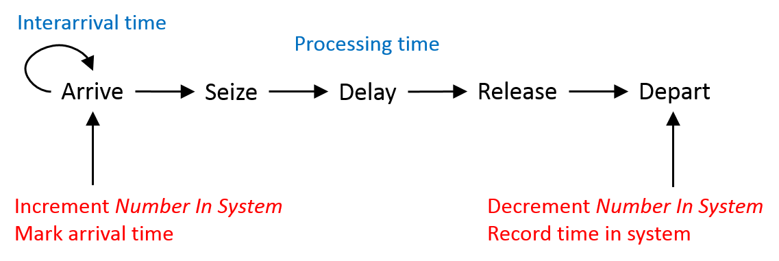
Figure 4.13: Basic process for the seize-delay-release model.

For our single-server queueing model, we simply set \(c=1\) and \(s=1\) (for all entities). So our single-server model is just an implementation of the basic seize-delay-release logic illustrated in Figure 4.13. Creating this model using processes is a little bit more involved than it was using Standard Library Objects, but it’s instructive to go through the model development and see the mechanisms for collecting user-defined statistics. Figure 4.14 shows the completed Simio process.

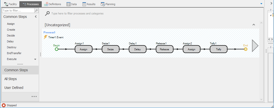
Figure 4.14: Process view of Model 4-2.

The steps to implement this model in Simio (see ) are as follows:

1. Open Simio and create a new model.

2. Create a Resource object in the Facility Window by dragging a Resource object from the Standard Library onto the Facility Window. In the Process Logic section of the object’s properties, verify that the Initial Capacity Type is Fixed and that the Capacity is 1 (these are the defaults). Note the object Name in the General section (the default is Resource1).

3. Make sure that the Model is highlighted in the Navigation Window and switch to the Definitions Window by clicking on the Definitions tab and choose the States section by clicking on the corresponding panel icon on the left. This prepares us to add a state to the model.

4. Create a new discrete (integer) state by clicking on the Integer icon in the States ribbon. Change the default Name property of IntegerState1 for the state to WIP. Discrete States are used to record numerical values. In this case, we’re creating a place to store the current number of entities in the model by creating an Integer Discrete State for the model (the Number In System from Figure 4.13).

5. Switch to the Elements section by clicking on the panel icon and create a Timer element by clicking on the Timer icon in the Elements ribbon (see Figure 4.15). The Timer element will be used to trigger entity arrivals (the loop-back arc in Figure 4.13). In order to have Poisson arrivals at the rate of \(\lambda=48\) entities/hour, or equivalently exponential interarrivals with mean \(1/0.8 = 1.25\) minutes, set the Time Interval property to Random.Exponential(1.25) and make sure that the Units are set to Minutes.

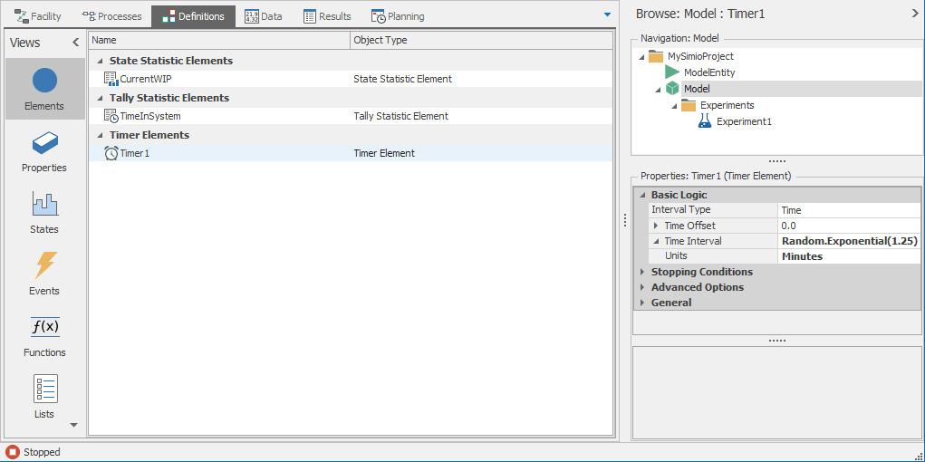
Figure 4.15: Timer element for the Model 4-2.

6. Create a State Statistic by clicking on the State Statistic icon in the Statistics section of the Elements ribbon. Set the State Variable Name property to WIP (the previously defined model Discrete State so it appears on the pull-down there) and set the Name property to CurrentWIP. We’re telling Simio to track the value of the state over time and record a time-dependent statistic on this value.

7. Create a Tally Statistic by clicking on the Tally Statistic icon in the Statistics section of the Elements ribbon. Set the Name property to TimeInSystem and set the Unit Type property to Time. Tally Statistics are used to record observational (i.e., discrete-time) statistics.

8. Switch to the Process Window by clicking on the Processes tab and create a new Process by clicking on the Create Process icon in the Process ribbon.

9. Set the Triggering Event property to be the newly created timer event (see Figure 4.16). This tells Simio to execute the process whenever the timer goes off.

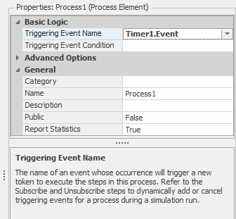
Figure 4.16: Setting the triggering event for the process.

10. Add an Assign step by dragging the Assign step from the Common Steps panel to the process, placing the step just to the right of the Begin indicator in the process. Set the State Variable Name property to WIP and the New Value property to WIP + 1, indicating that when the event occurs, we want to increment the value of the state variable to reflect the fact that an entity has arrived to the system (the “Increment” in Figure 4.13).

11. Next, add the Seize step to the process just to the right of the Assign step. To indicate that Resource1 should be seized by the arriving entity, click the ... button on the right and select the Seizes property in the Basic Logic section, click Add, and then indicate that the specific resource Resource1 should be seized (see Figure 4.17).

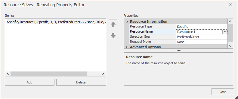
Figure 4.17: Setting the Seize properties to indicate that Resource1 should be seized.

12. Add the Delay step immediately after the Seize step and set the Delay Time property to Random.Exponential(1) minutes to indicate that the entity delays should be exponentially distributed with mean \(1\) minute (equivalent to the original service rate of 60/hour).

13. Add the Release step immediately after the Delay step and set the Releases property to Resource1.

14. Add another Assign step next to the Release step and set the State Variable Name property to WIP and the New Value property to WIP - 1, indicating that when the entity releases the resource, we want to decrement the value of the state variable to reflect the fact that an entity has left the system.

15. Add a Tally step and set the TallyStatisticName property to TimeInSystem (the Tally Statistic was created earlier so is available on the pull-down there), and set the Value property to TimeNow - Token.TimeCreated to indicate that the recorded value should be the current simulation time minus the time that the current token was created. This time interval represents the time that the current entity spent in the system. The Tally step implements the Record function shown in Figure 4.13. Note that we used the token state Token.TimeCreated instead of marking the arrival time as shown in Figure 4.13.

16. Finally, switch back to the Facility Window and set the run parameters (e.g., set the Ending Type to a Fixed run length of 1000 hours).

Note that we’ll discuss the details of States, Properties, Tokens, and other components of the Simio Framework in Chapter 5.

To test the model, create an Experiment by clicking on the New Experiment icon in the Project Home ribbon. Figure 4.18 shows the Pivot Grid results for a run of 10 replications of the model using a 500 hour warm-up period for each replication. Notice that the report includes the UserSpecified category including the CurrentWIP and TimeInSystem statistics. Unlike the ModelEntity statistics NumberInSystem and TimeInSystem that Simio collected automatically in the Standard Library object model from Section 4.2, we explicitly told Simio to collect these statistics in the process model. Understanding user-specified statistics is important, as it’s very likely that you’ll want more than the default statistics as your models become larger and more complex. The CurrentWIP statistic is an example of a time-dependent statistic. Here, we defined a Simio state (step 4), used the process logic to update the value of the state when necessary (step 10 to increment and step 14 to decrement), and told Simio to keep track of the value as it evolves over simulated time and to report the summary statistics (of \(\widehat{L}\), in this case — step 4). The TimeInSystem statistic is an example of an observational or tally statistic. In this case, each arriving entity contributes a single observation (the time that entity spends in the system) and Simio tracks and reports the summary statistics for these values (\(\widehat{W}\), in this case). Step 7 sets up this statistic and step 15 records each observation.

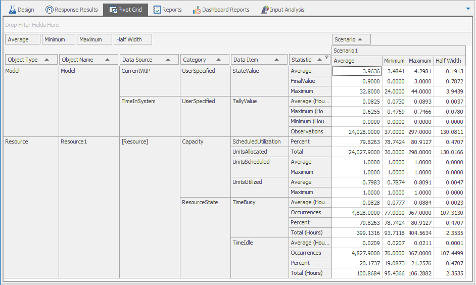
Figure 4.18: Results from Model 4-2.

Another thing to note about our processes model is that it runs significantly faster than the corresponding Standard Library objects model (to see this, simply increase the run length for both models and run them one after another). The speed difference is due to the overhead associated with the additional functionality provided by the Standard Library objects (such as automatic collection of statistics, animation, collision detection on paths, resource failures, etc.).

As mentioned above, most Simio models that you build will use the Standard Library objects and it’s unlikely that you’ll build complete models using only Simio processes. However, processes are fundamental to Simio and it is important to understand how they work. We’ll revisit this topic in more detail in Section 5.1.4, but for now we’ll return to our initial model using the Standard Library objects.

4.4 Model 4-3: Automated Teller Machine (ATM)

In developing our initial Simio models, we focused on an arbitrary queueing system with entities and servers — very boring. Our focus for this section and for Section 4.8 is to add some context to the models so that they’ll more closely represent the types of “real” systems that simulation is used to analyze. We’ll continue to enhance the models over the remaining chapters in this Part of the book as we continue to describe the general concepts of simulation modeling and explore the features of Simio. In Models 4-1 and 4-2 we used observations from the exponential distribution for entity inter-arrival and service times. We did this so that we could exploit the mathematical “niceness” of the resulting \(M/M/1\) queueing model in order to demonstrate the basics of randomness in simulation. However, in many modeling situations, entity inter-arrivals and service times don’t follow nice exponential distributions. Simio and most other simulation packages can sample from a wide variety of distributions to support general modeling. Models 4-3 and 4-4 will demonstrate the use of a triangular distribution for the service times, and the models in Chapter 5 will demonstrate the use of many of the other standard distributions. Section 6.1 discusses how to specify such input probability distributions in practice so that your simulation model will validly represent the reality you’re modeling.

Model 4-3 models the automated teller machine (ATM) shown in Figure 4.19. Customers enter through the door marked Entrance, walk to the ATM, use the ATM, and walk to the door marked Exit and leave. For this model, we’ll assume that the room containing the ATM is large enough to handle any number of customers waiting to use the ATM (this will make our model a bit easier, but is certainly not required and we’ll revisit the use of limited-capacity queues in future chapters). With this assumption, we basically have a single-server queueing model similar to the one shown in Figure 4.1. As such, we’ll start with Model 4-1 and modify the model to get our ATM model (be sure to use the Save Project As option to save Model 4-3 initially so that you don’t over-write your file for Model 4-1). The completed ATM model (Model 4-3) is shown in Figure 4.20.

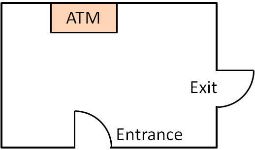
Figure 4.19: ATM example.

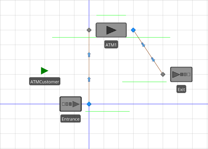
Figure 4.20: Model 4-3: ATM example.

The required modifications are as follows:

1. Update the object names to reflect the new model context (ATMCustomer for entities, Entrance for the Source object, ATM1 for the Server object, and Exit for the Sink object);

2. Rearrange the model so that it “looks” like the figure;

3. Change the Connector and entity objects so that the model includes the customer walk time; and

4. Change the ATM processing-time distribution so that the ATM transaction times follow a triangular distribution with parameters (0.25, 1.00, 1.75) minutes (that is, between 0.25 and 1.75 minutes, with a mode of 1.00 minute).

Updating the object names doesn’t affect the model’s running characteristics or performance, but naming the objects can greatly improve model readability (especially for large or complicated models). As such, you should get into the habit of naming objects and adding meaningful descriptions using the Description property. Renaming objects can be done by either selecting the object, hitting the F2 key, and typing the new name; or by editing the Name property for the object. Rearranging the model to make it look like the system being modeled is very easy — Simio maintains the connections between objects as you drag the object around the model. Note that in addition to moving objects, you can also move the individual object input and output nodes.

In our initial queueing model (Model 4-1) we assumed that entities simply “appeared’’ at the server upon arrival. The Simio Connector object supported this type of entity transfer. This is clearly not the case in our ATM model where customers walk from the entrance to the ATM and from the ATM to the exit (most models of”real” systems involves some type of similar entity movement). Fortunately, Simio provides several objects from the Standard Library to facilitate modeling entity movements:

• Connector — Transfers entities between objects in zero simulation time (i.e., instantly, at infinite speed);

• Path — Transfers entities between objects using the distance between objects and entity speed to determine the movement time;

• TimePath — Transfers entities between objects using a user-specified movement-time expression; and

• Conveyor — Models physical conveyors.

We’ll use each of these methods over the next few chapters, but we’ll use Paths for the ATM model (note that the Simio Reference Guide, available via the F1 key or the ? icon in the upper right of the Simio window, provides detailed explanations of all of these objects). Since we’re modifying Model 4-1, the objects are already connected using Connectors. The easiest way to change a Connector to a Path is to right-click on the Connector and choose the Path option from the Convert to Type sub-menu. This is all that’s required to change the connection type. Alternatively, we could delete the Connector object and add the Path object manually by clicking on the Path in the Standard Library and then selecting the starting and ending nodes for the Path.

The entity-movement time along a Path object is determined by the path length and the entity speed. Simio models are drawn to scale by default so when we added a path between two nodes, the length of the path was set as the distance between the two nodes (whenever you input lengths or other properties with units, the + will expand a field where you can specify the input units. The Unit Settings button on the Run ribbon allows you to change the units displayed on output, such as in the facility-window labels, the pivot-grid numbers, and trace output). The Length property in the Physical Characteristics/Size group of the General section gives the current length of the Path object. The length of the path can also be estimated using the drawing grid. The logical path length can also be manually set if it’s not convenient to draw the path to scale. To set the logical length manually, set the Drawn to Scale property to False and set the Logical Length property to the desired length. The entity speed is set through the Initial Desired Speed property in the Travel Logic section of the entity properties. In Model 4-3, the path length from the entrance to the ATM is 10 meters, the path length from the ATM to the exit is 7 meters, and the entity speed is 1 meter/second. With these values, an entity requires 10 seconds of simulated time to move from the entrance to the ATM, and 7 seconds to move from the ATM to the exit. The path lengths and entity speed can be easily modified as dictated by the system being modeled.

The final modification for our ATM model involves changing the processing-time distribution for the server object. The characteristics of the exponential distribution probably make it ill-suited for modeling the transaction or processing time at an ATM. Specifically, the exponential distribution is characterized by lots of relatively small values and a few extremely large values, since the mode of its density function is zero. Given that all customers must insert their ATM card, correctly enter their personal identification number (PIN), and select their transaction, and that the number of ATM transaction types is generally limited, a bounded distribution is likely a better choice. We’ll use a triangular distribution with parameters 0.25, 1.00, and 1.75 minutes. Determining the appropriate distribution(s) to use is part of input analysis, which is covered in Section 6.1. For now, we’ll assume that the given distributions are appropriate. To change the processing-time distribution, simply change the Processing Time property to Random.Triangular(0.25, 1, 1.75) and leave the Units property as Minutes. By using the Random keyword, we can sample statistically independent observations from some 19 common distributions (as of the writing of this book) along with the continuous and discrete empirical distributions for cases where none of the standard distributions provides an adequate fit. These distributions, their required parameters, and plots of their density or probability-mass functions are discussed in detail in the “Distributions’’ subsection of the”Expressions Editor, Functions and Distributions” section in the “Modeling in Simio” part of the Simio Reference Guide. The computational methods that Simio uses to generate random numbers and random variates are discussed in Sections 6.3 and 6.4.

Now that we have completed Model 4-3, we must verify our model as discussed in Section 4.2.5. As noted, the verification process involves developing a set of expectations, developing and running the model, and making sure that the model results match our expectations. When there’s a mismatch between our expectations and the model results, we must find and fix the problems with the model, the expectations, or both. For Model 4-1, the process of developing expectations was fairly simple — we were modeling an \(M/M/1\) queueing system so we could calculate the exact values for the performance metrics. The process isn’t quite so simple for Model 4-3, as we no longer have exponential processing times, and we’ve added entity-transfer times between the arrival and service, and between the service and the departure. Moreover, these two modifications will tend to counteract each other in terms of the queueing metrics. More specifically, we’ve reduced the variation in the processing times, so we’d expect the numbers of entities in system and in the queue as well as the time in system to go down (relative to Model 4-1), but we’ve also added the entity-transfer times, so we’d expect the number of entities in the system and the time that entities spend in the system to go up. As such, we don’t have a set of expectations that we can test. This will be the case quite often as we develop more complex models. Yet we’re still faced with the need for model verification.

One strategy is to develop a modified model for which we can easily develop a set of expectations and to use this modified model during verification. This is the approach we’ll take with Model 4-3. There are two natural choices for modifying our model: Set the Entity Transfer Times to 0 and use an \(M/G/1\) queueing approximation (as described in Chapter 2), or change the processing-time distribution to exponential. We chose the latter option and changed the Processing Time property for the ATM to Random.Exponential(1). Since we’re simply adding 17 seconds of transfer time to each entity, we’d expect \(\rho\), \(L_q\), and \(W_q\) to match the \(M/M/1\) values (Table 4.2), and \(W\) to be 17 seconds greater than the corresponding \(M/M/1\) value. The results for running 500 replications of our model with replication length 30 hours and warm-up of 20 hours (the same conditions as we used in Section 4.2.5) are given in Table 4.6.

Table 4.6: Model 4-3 (modified version) results.

Metric being estimated	Simulation
Utilization (\(\rho\))	\(0.797 \pm 0.004\)
Number in system (\(L\))	\(4.139 \pm 0.131\)
Number in queue (\(L_q\))	\(3.115 \pm 0.128\)
Time in system (\(W\))	\(0.086 \pm 0.003\)
Time in queue (\(W_q\))	\(0.064 \pm 0.003\)

These results appear to match our expectations (we could run each replication longer or run additional replications if we were concerned with the minor deviations between the average values and our expectations, but we’ll leave this to you). So if we assume that we have appropriately verified the modified model, the only way that Model 4-3 wouldn’t be similarly verified is if either we mistyped the Processing Time property, or if Simio’s implementation of either the random-number generator or Triangular random-variate generator doesn’t generate valid values. At this point we’ll make sure that we’ve entered the property correctly, and we’ll assume that Simio’s random-number and random-variate generators work. Table 4.7 gives the results of our experiment for Model 4-3 (500 replications, 30 hours run length, 20 hours warm-up). As expected, the number of entities in the queue and the entities’ time in system have both gone down (this was expected since we’ve reduced the variation in the service time). It’s worth reiterating a point we made in Section 4.2.5: We can’t (in general) prove that a model is verified. Instead, we can only collect evidence until we’re convinced (possibly finding and fixing errors in the process).

Table 4.7: Model 4-3 results.

Metric being estimated	Simulation
Utilization (\(\rho\))	\(0.800 \pm 0.003\)
Number in system (\(L\))	\(2.791 \pm 0.064\)
Number in queue (\(L_q\))	\(1.764 \pm 0.061\)
Time in system (\(W\))	\(0.058 \pm 0.001\)
Time in queue (\(W_q\))	\(0.036 \pm 0.001\)

4.5 Beyond Means: Simio MORE (SMORE) Plots

We’ve emphasized already in several places that the results from stochastic simulations are themselves random, so need to be analyzed with proper statistical methods. So far, we’ve tended to focus on means — using averages from the simulation to estimate the unknown population means (or expected values of the random variables and distributions of the output responses of interest). Perhaps the most useful way to do that is via confidence intervals, and we’ve shown how Simio provides them in its Experiment Pivot Grids and Reports. Means (of anything, not just simulation-output data) are important, but seldom do they tell the whole tale since they are, by definition, the average of an infinite number of replications of the random variable of interest, such as a simulation output response like average time in system, maximum queue length, or a resource utilization, so don’t tell you anything about spread or what values are likely and unlikely. This is among the points made by Sam Savage in his engagingly-titled book, The Flaw of Averages: Why We Underestimate Risk in the Face of Uncertainty (Savage 2009). In the single-period static inventory simulation of Section 3.2.3, and especially in Figure 3.3, we discussed histograms of the results, in addition to means, to see what kind of upside and downside risk there might be concerning profit, and in particular the risk that there might be a loss rather than a profit. Neither of these can be addressed by averages or means since, for example, if we order 5000 hats, the mean profit seemed likely to be positive (95% confidence interval \(\$8734.20 \pm \$3442.36\)), yet there was a 30% risk of incurring a loss (negative profit).

So in addition to the Experiment Pivot Grid and Report, which contain confidence-interval information to estimate means, Simio includes a new type of chart for reporting output statistics. Simio MORE (SMORE) plots are a combination of an enhanced box plot, first described by John Tukey in 1977 (Tukey 1977), a histogram, and a simple dot plot of the individual-replication summary responses. SMORE plots are based on the Measure of Risk and Error (MORE) plots developed by Barry Nelson in (B. L. Nelson 2008), and Figure 4.21 shows a schematic defining some of their elements. A SMORE plot is a graphical representation of the run results for a summary output performance measure (response), such as average time in system, maximum number in queue, or a resource utilization, across multiple replications. Similar to a box plot in its default configuration, it displays the minimum and maximum observed values, the sample mean, sample median, and “lower” and “upper” percentile values (points at or below which are that percent of the summary responses across the replications). The “sample” here is composed of the summary measures across replications, not observations from within replications, so this is primarily intended for terminating simulations that are replicated multiple times, or for steady-state simulations in which appropriate warm-up periods have been identified and the model is replicated with this warm-up in effect for each replication. A SMORE plot can optionally display confidence intervals on the mean and both lower/upper percentile values, a histogram of observed values, and the responses from each individual replication.

Figure 4.21: SMORE plot components (from the Simio Reference Guide).

SMORE plots are generated automatically based on experiment Responses. For Model 4-3, maybe we’re interested in the average time, over a replication, that customers spend in the system (the time interval between when a customer arrives to the ATM and when that customer leaves the ATM). Simio tracks this statistic automatically and we can access within-replication average values as the expression ATMCustomer.Population.TimeInSystem.Average. To add this as a Response, click the Add Response icon in the Design ribbon (from the Experiment window) and specify the Name (AvgTimeInSystem) to label the output, and Expression (ATMCustomer.Population.TimeInSystem.Average) properties (see Figure 4.22). A reasonable question you might be asking yourself right about now is, “How do I know to type in ATMCustomer.Population.TimeInSystem.Average there for the Expression?” Good question, but Simio provides a lot of on-the-spot, smart, context-sensitive help.

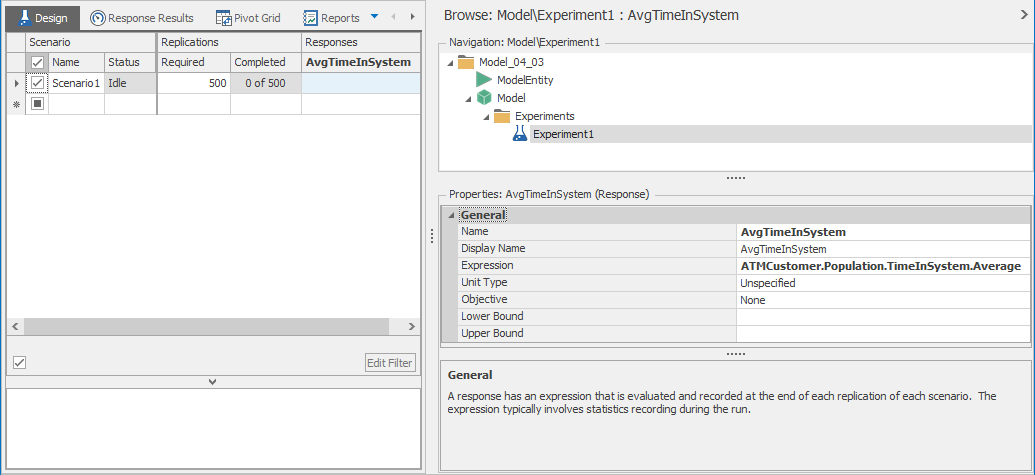
Figure 4.22: Defining the experiment Response for average time in system in Model 4-3.

When you click in the Expression field you’ll see a down arrow on the right; clicking it brings up another field with a red X and green check mark on the right — this is Simio’s expression builder, discussed more fully in Section 5.1.7, and shown in Figure 4.23.

Figure 4.23: Using the Simio expression builder for the average-time-in-system Response for a SMORE plot.

For now, just experiment with it, starting by clicking in the blank expression field and then tapping the down-arrow key on your keyboard to open up a menu of possible ways to get started, at the left edge of the expression. In the list that appears below, find ATMCustomer (since that’s the name of the entities, and we want something about entities here, to wit, their time in system) and double-click on it; note that that gets copied up into the expression field. Next, type a period just to the right of ATMCustomer in the expression field, and notice that another list drops down with valid possibilities for what comes next. In this case we are looking for a statistic for the entire population of ATMCustomer entities, not just a particular entity, so double-click on Population. Again you are provided a list of choices; double-click on TimeInSystem at the bottom of the list (since that’s what we want to know about our ATMCustomer entities). If at any point you lose your drop-down list, just type the down arrow again. As before, type a period on the right of the expression that’s gradually getting built in the field, and double-click on Average in the list that appears (since we want the average time in system of ATMCustomer entities, rather than the maximum or minimum — though the latter two would be valid choices if you wanted to know about them rather than the average). That’s the end of it, as you can verify by trying another period and down arrow but nothing happens, so click on the green check mark on the right to establish this as your expression.

You can add more Responses in this way, repeatedly clicking on the Add Response icon and filling in the Properties as above, and when viewing the SMORE plots you can rotate among them via a drop-down showing the Names you chose for them. Go ahead and add two more: the first with Name = MaxQueueLength and Expression = ATM1.AllocationQueue.MaximumNumberWaiting, and the second with Name = ResourceUtilization and Expression = ATM1.ResourceState.PercentTime(1). We invite you to poke through the expression builder to discover these, and in particular the (1) in the last one (note that as you hover over selections in the drop-downs from the expression builder, helpful notes pop up, as in Figure 4.23, describing what the entries are, including the (1)). The percents desired for the Lower and Upper Percentiles, and the Confidence Level for the confidence intervals can be set using the corresponding experiment properties (see Figure 4.24); by default, the lower and upper percentiles are set for 25% and 75% (i.e., the lower and upper quartiles) as in traditional box plots, though you may want to spread them out more than that since the “box” to which your eye is drawn contains the results from only the middle half of the replications in the default traditional settings, and maybe you’d like your eye to be drawn to something that represents more than just half (e.g., setting them at 10% and 90% would result in a box containing 80% of the replications’ summary results).

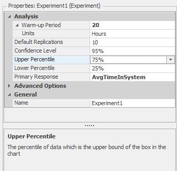
Figure 4.24: Setting the percentile and confidence interval levels.

To view your SMORE plots, select the Response Results tab in the Experiment window. Figure 4.25 shows the SMORE plot for the average time in system from a 500-replication run of Model 4-3 described above (30-hour run length, 20-hour warm-up on each replication), with the Confidence Intervals and Histogram showing, but not the individual replication-by-replication observations. We left the percentiles at their defaults of 75% for upper and 25% for lower. The Rotate Plot button allows you to view the plot horizontally rather than vertically, if you prefer. The numerical values used to generate the SMORE plot, like the confidence-interval endpoints, are also available by clicking on the Raw Data tab at the bottom of the SMORE plot window, so you can see what they actually are rather than eyeballing them from the graph. We see from Figure 4.25 that the expected average time in system is just under 0.058 hour (3.5 minutes), and the median is a bit lower, consistent with the histogram shape’s being skewed to the right. Further, the upper end of the box plot (75th percentile) is about 0.064 hour (3.8 minutes), so there’s a 25% chance that the average time in system over a replication will be more than this. And the confidence-intervals seem reasonably tight, indicating that the 500 replications we made are enough to form reasonably precise conclusions.

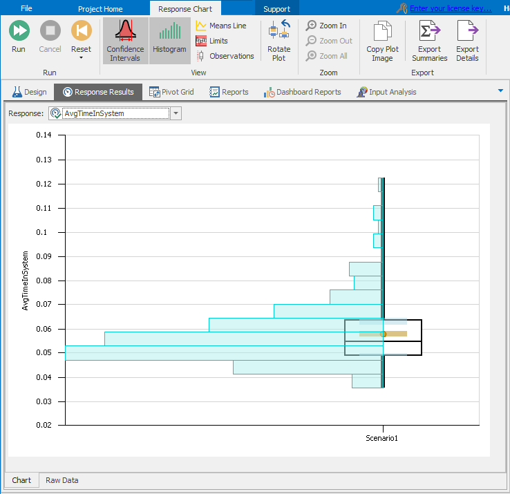
Figure 4.25: SMORE plot for average time in system in Model 4-3.

Figure 4.26 shows the SMORE plots (with the same elements showing) for the maximum queue length; we temporarily moved the Upper Percentile from its default 75% up to 90%. Since this is for the maximum (not average) queue length across each replication, this tells us how much space we might need to hold this queue over a whole replication, and we see that if we provide space for 14 or 15 people in the ATM lobby, we’ll always (remember, we’re looking at the maximum queue length) have room to hold the queue in about 90% of the replications. Play around a bit with the Upper Percentile and Lower Percentile settings in the Experiment Design window; of course, as these percentiles move out toward the extreme edges of 0% and 100%, the edges of the box move out too, but what’s interesting is that the Confidence Intervals on them become wider, i.e., less precise. This is because these more extreme percentiles are inherently more variable, being based on only the paucity of points out in the tails, and are thus more difficult to estimate, so the wider confidence intervals keep you honest about what you know (or, more to the point, what you don’t know) concerning where the true underlying percentiles really are.

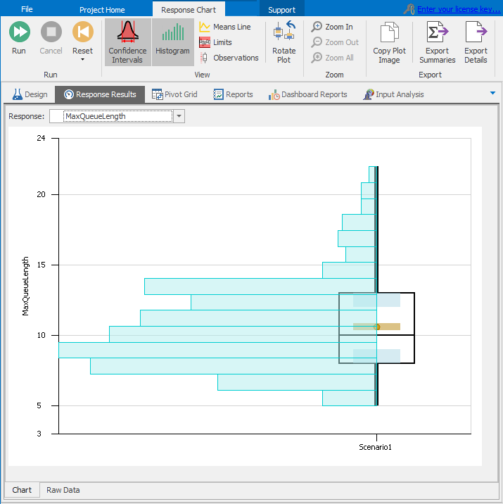
Figure 4.26: SMORE plot for maximum queue length in system in Model 4-3.

The distribution of the observed server utilization in Figure 4.27 shows that it will be between 77% and 83% about half the time, which agrees with the queueing-theoretic expected utilization of \[ \frac{\mbox{E(service time)}}{\mbox{E(interarrival time)}} = \frac{(0.15 + 1.00 + 1.75)/3}{1.25} = 0.80 \] (the expected value of a triangular distribution with parameters min, mode, max is (min + mode + max)/3, as given in the Simio Reference Guide). However, there’s a chance that the utilization could be as heavy as 90% since the histogram extends up that high (the maximum utilization across the 500 replications was 90.87%, as you can see in the Raw Data tab at the bottom).

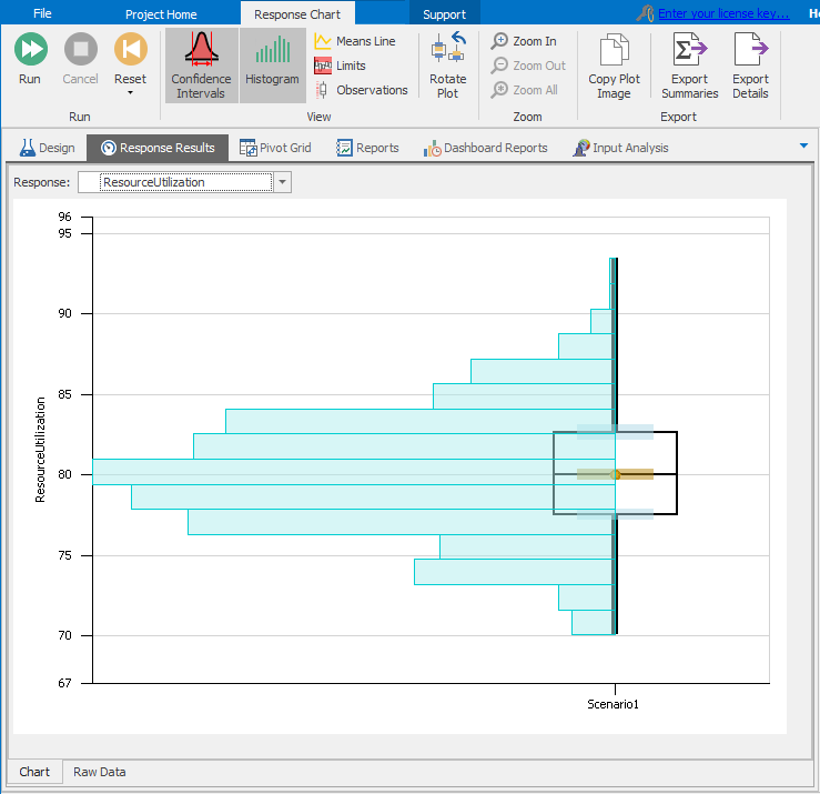
Figure 4.27: SMORE plot for server utilization in Model 4-3.

As originally described in (B. L. Nelson 2008), SMORE plots provide an easy-to-interpret graphical representation of a system’s risk and the sampling error associated with the simulation — far more information than just the average over the replications, or even a confidence interval around that average. The confidence intervals in a SMORE plot depict the sampling error in estimation of the percentiles and mean — we can reduce the width of the confidence intervals (and, hence, the sampling error) by increasing the number of replications. Visually, if the confidence-interval bands on the SMORE plot are too wide to suit you, then you need to run more replications. Once the confidence intervals are sufficiently narrow (i.e., we’re comfortable with the sampling error), we can use the upper and lower percentile values to get a feeling for the variability associated with the response. We can also use the histogram to get an idea about the distribution shape of the response (e.g., in Figures 4.25-\(\ref{fig:model-4-3-smore-util}\) it’s apparent that the distributions of average time in system and maximum queue length are skewed right or high, but the distribution of utilizations is fairly symmetric). As we’ll see in Chapter 5, SMORE plots are quite useful to see what the differences might be across multiple alternative scenarios in an output performance measure, not only in terms of just their means, but also their relative spread and distribution.

4.6 Exporting Output Data for Further Analysis

Simio is a simulation package, not a statistical-analysis package. While it does provide some statistical capabilities, like the confidence intervals and SMORE plots that we’ve seen (and a few more that we’ll see in future chapters), Simio makes it easy to export the results of your simulation to a CSV file that can then be easily read into a variety of dedicated statistical-analysis packages like SAS, JMP, SPSS, Stata, S-PLUS, or R, among many, many others, for post-processing your output data after your simulations have run. For relatively simple statistical analysis, the CSV file that you can ask Simio to export for you can be read directly into Excel and you could then use its built-in functions (like =AVERAGE, =STDEV, etc.) or the Data Analysis Toolbar that comes with Excel, or perhaps a better and more powerful third-party statistical-analysis add-in like StatTools from Palisade Corporation. With your responses from each replication exported in a convenient format like this, you’re then free to use your favorite statistics package to do any analysis you’d like, such as hypothesis tests, analysis of variance, or regressions. Remember, from each replication you get a single summary value (e.g., average time in system, maximum queue length, or server utilization over the replication), not individual-entity results from within replications, and those summary values are independent and identically distributed observations to which standard statistical methods will apply; your “sample size,” in statistics parlance, is the number of replications you ran. Note that you can collect individual-entity observations manually with a Write step in add-on process logic or with simple customization of a standard library object as described in Section 11.4. You can also enable logs to collect tally and state statistic observations and Dashboard Reports to display them.

You’ve already seen how this export to a CSV file can be done, in Section 4.2.3, from the Experiment window via the Export Details icon in the Pivot Grid window. Depending on the size of your model, and the number of replications you made, this exported CSV file could be fairly large, and you may need to do some rearranging of it, or extracting from it, to get at the results you want. But once you have the numbers you want saved in this convenient format, you can do any sort of statistical analysis you’d like, including perhaps data mining to try to discover patterns and relationships from the output data themselves.

For example, in the 500 replications we used to make the SMORE plots in Section 4.5, we exported the data and extracted the 500 average times in system to one column in an Excel spreadsheet, and the 500 utilizations in a second column. Thus, in each of the 500 rows, the first-column value is the average time in system on that replication, and the second-column value is the server utilization in that same replication. We then used the StatTools statistical-analysis add-in to produce the scatterplot and correlation in Figure 4.28.

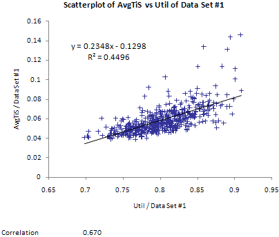
Figure 4.28: StatTools scatterplot of average time in system vs. server utilization in Model 4-3.

We see that there’s some tendency for average time in system to be higher when the server utilization is higher, but there are plenty of exceptions to this since there is a lot of random “noise” in these results. We also used the built-in Excel Chart Tools to superpose a linear regression line, and show its equation and \(R^2\) value, confirming the positive relationship between average time in system and server utilization, with about 45% of the variation in average time in system’s being explained by variation in server utilization. This is just one very small example of what you can do by exporting the Simio results to a CSV file, extracting from it appropriately (maybe using custom macros or a scripting language), and then reading your simulation output data into powerful statistical packages to learn a lot about your models’ behavior and relationships.

4.7 Interactive Logs and Dashboard Reports

Simio provides capabilities for logging various data during interactive runs and using this data to create dashboard reports. All Simio license types provide limited logging capabilities; Academic RPS licenses provide additional related capabilities. Note that Simio’s logging and dashboard features are quite extensive and we will only demonstrate a simple case here. Additional feature descriptions and details are available in the Simio Help and SimBits.

For this example, we will use Model 4-3 and will log the ATM resource usage and create a related dashboard report. First we will tell Simio to log the resource usages for the ATM server resource. The steps to do this are as follows:

1. Turn on interactive logging from the Advanced Options item on the Run ribbon.

2. Turn on resource usage logging for the ATM server object. To do this, select the ATM object instance, expand the Advanced Options resource group and set the Log Resource Usage property to True.

3. Reset and run the model in fast-forward mode.

4. Navigate to the Logs section of the Results tab and select the Resource Usage Log (if it is not already selected). Figure 4.29 shows a portion of the the Resource Usage Log view for the newly created log.

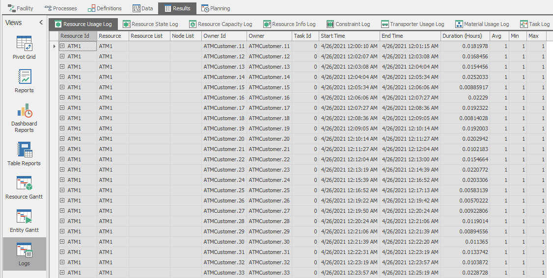
Figure 4.29: Resource Usage Log for Model 4-3.

The resource usage log records every time the specified resource is “used” and specifies the entity, the start time, the end time, and duration of the usage. Now that the individual resource usages are logged, we will create a simple dashboard report that plots the usage durations over the simulation time. The steps are as follows:

1. Select the Dashboard Reports section of the Results tab, click on the Create item from the Dashboards ribbon, and enter a name for your dashboard in the Add Dashboard dialog box. Figure 4.30 shows the initial dialog box for the new dashboard. Select the Resource Usage Log from the Data Source drop-box.

Figure 4.30: Initial dialog box for the new dashboard report.

2. Click on the Chart option from the Chart Tools/Home ribbon to create a new chart. Figure 4.31 shows the the newly created chart in the new dashboard report. From here, we customize the chart by dragging items from the Resource Usage Log and dropping them on the DATA ITEMS components.

Figure 4.31: Newly created chart for the dashboard.

3. Drag the Duration (Hours) item and drop it on the Values (Pane 1) data item.

4. Click on the bar chart item just to the right of the data item and change the chart type to a line plot.

5. Drag the Start Time item and drop it on the Arguments data item.

6. Open the drop-box for the data source and select the Date-Hour-Minute option from the list. Figure 4.32 shows the the completed resource usage chart. The chart plots the resource usage durations by the start time of the usages.

Figure 4.32: Final resource usage chart for the dashboard.

7. Click the Save item on the ribbon to save the newly created dashboard.

As mentioned, Simio’s logging and dashboard capabilities are extensive and you should experiment with these features and have a look at the Simio Help and related SimBits. In addition, details, examples, and instructions about Dashboards are available in the Simio help and at https://docs.devexpress.com/Dashboard/.

4.8 Basic Model Animation

Up until now we’ve barely mentioned animation, but we’ve already been creating useful animations. In this section we’ll introduce a few highlights of animation. We’ll cover animation in much greater detail in Chapter 8. Animation generally takes place in the Facility Window. If you click in the Facility Window and hit the H key, it will toggle on and off some tips about using the keyboard and mouse to move around the animation. You might want to leave this enabled as a reminder until you get familiar with the interface.

One of Simio’s strengths is that when you build models using the Standard Library, you’re building an animation as you build the model. The models in Figures 4.8 and 4.20 are displayed in two-dimensional (2D) animation mode. Another of Simio’s strengths is that models are automatically created in 3D as well, even though the 2D view is commonly used during model building. To switch between 2D and 3D view modes, just tap the 2 and 3 keys on the keyboard, or select the View ribbon and click on the 2D or 3D options. Figure 4.33 shows Model 4-3 in 3D mode. In 3D mode, the mouse buttons can be used to pan, zoom, and rotate the 3D view. The model shown in Figure 4.33 shows one customer entity at the server (shown in the Processing.Contents queue attached to the ATM1 object), five customer entities waiting in line for the ATM (shown in the InputBuffer.Contents queue for the ATM1 server object), and two customers on the path from the entrance to the ATM queue.

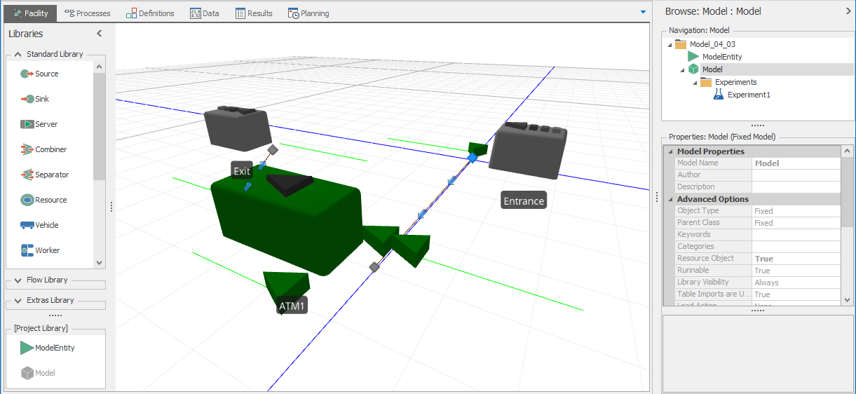
Figure 4.33: Model 4-3 in 3D view.

Let’s enhance our animation by modifying Model 4-3 into what we’ll call Model 4-4. Of course, you should start by saving Model_04_03.spfx to a file of a new name, say Model_04_04.spfx, and maybe to a different directory on your system so you won’t overwrite our file of the same name that you might have downloaded; Simio’s Save As capability is via the yellow pull-down tab just to the left of the Project Home tab on the ribbon.

If you click on any symbol or object, the Symbols ribbon will come to the front. This ribbon provides options to change the color or texture applied to the symbol, add additional symbols, and several ways to select a symbol to replace the default. We’ll start with the easiest of these tasks — selecting a new symbol from Simio’s built-in symbol library. In particular, let’s change our entity picture from the default green triangle to a more realistic-looking person.

Start by clicking on the Entities object we named ATMCustomer. In the Symbols ribbon now displayed, if you click the Apply Symbols button, you will see the top section of the built-in library as illustrated in Figure 4.34.

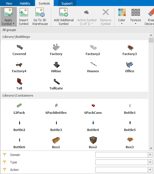
Figure 4.34: Navigating to Simio symbol library.

The entire library consists of over 300 symbols organized into 27 categories. To make it easier to find a particular symbol, three filters are supplied at the bottom: Domain, Type, and Action. You can use any combination of these filters to narrow the choices to what you are looking for. For example, let’s use the Type filter and check only the People option, resulting in a list of all the People in the library. Near the top you will see a Library People category. If you hover the mouse (don’t click yet) over any symbol, you’ll see an enlarged view to assist you with selection. Click on one of the “Female” symbols to select it and apply it as the new symbol to use for your highlighted object — the entity. The entity in your model should now look similar to that in Figure 4.35. Note that under the People folder there is an folder named Animated that contains symbols of people with built-in animation like Walking, Running, and Talking. Using these provides even more realistic animation, but that is probably overkill for our little ATM model.

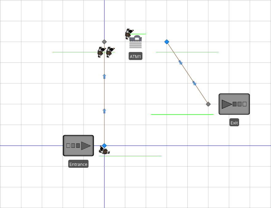
Figure 4.35: Model 4-4 with woman and ATM symbols in 2D view.

You may notice that Figure 4.35 also contains a symbol for an ATM machine. Unfortunately this was not one of the symbols in the library. If you happened to have an ATM symbol readily available you could import it. Or if you’re particularly artistic you could draw one. But for the rest of us Simio provides a much easier solution — download it from Trimble 3D Warehouse. This is a huge repository of symbols that are available free, and Simio provides a direct link to it. Let’s change the picture of our server to that of an ATM machine.

Start by clicking on the Server object we’d previously named ATM1. Now go to the Symbol ribbon and click on the Go To 3D Warehouse icon. This will open the 3D Warehouse web page (https://3dwarehouse.sketchup.com) in your default web browser. Enter ATM into the Search box and click on the Search button and then choose the Models tab. You’ll see the first screen of hundreds of symbols that have ATM in their name or description, something like Figure 4.36. Note that the library is updated frequently, so your specific search results may vary. Similarly, the web page may also look/behave differently if it has been updated since the writing of this chapter.

Figure 4.36: Trimble Warehouse results of search for ATM.

Note that many of these don’t involve automated teller machines, but many do, and in fact you should find at least one on the first screen that meets our needs. You can click on an interesting object (we chose a Mesin ATM) and see the basic details such as file size. If you click on the See more details link, you can view and rotate the model in 3D from the browser. If you are satisfied, choose Download and save the skp file on your computer (you may have to set up an account on the 3D warehouse site if you do not already have one in order to download symbols). Back in Simio, you can import the symbol and apply it to the selected Server using the Import Symbol icon (with the Server object instance selected). This will import the 3D model into your Simio model, allow you to change the name size and orientation of the symbol, and apply it to the object instance. Once the symbol has been imported, it can be applied to other object instances without re-importing (using the Apply Symbol icon).

One of the most important things to verify during the import process is that the size (in meters) is correct. You cannot change the ratio of the dimensions, but you can change any one value if it was sized wrong. In our case our ATM is about 0.7 meter wide and 2 meters high, which seems about right. Click OK and we’re done applying a new symbol to our ATM server. Now your new Model 4-4 should look something like to Figure 4.35 when running in the 2D view. If you change to the 3D view (3 key) you should see that those new symbols you selected also look good in 3D, as in Figure 4.37.

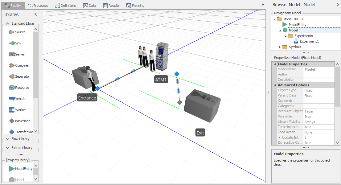
Figure 4.37: Model 4-4 with woman and ATM symbols in 3D view.

Of course we’ve barely scratched the surface of animation possibilities. You could draw walls (see the Drawing ribbon), or add features like doorways and plants. You can even import a schematic or other background to make your model look even more realistic. Feel free to experiment with such things now if you wish, but we’ll defer formal discussion of these topics until Chapter 8.

4.9 Model Debugging

As hard as it may be to believe, sometimes people make mistakes. When those mistakes occur in software they are often referred to as bugs. Many things can cause a bug including a typo (typing a 2 when you meant to type a 3), a misunderstanding of how the system works, a misunderstanding of how the simulation software works, or a problem in the software. Even the most experienced simulationist will encounter bugs. In fact a significant part of most modeling efforts is often spent resolving bugs — it is a natural outcome of using complex software to model complex systems accurately. It is fairly certain that you will have at least a few bugs in the first real model that you do. How effectively you recognize and dispatch bugs can determine your effectiveness as a modeler. In this section we will give you some additional insight to improve your debugging abilities.

The best way to minimize the impact of bugs is to follow proper iterative development techniques (see Section 1.5.3). If you work for several hours without stopping to verify that your model is running correctly, you should expect a complex and hard-to-find bug. Instead, pause frequently to verify your model. When you find problems you will have a much better idea of what caused the problem and you will be able to find and fix it much more quickly.

The most common initial reaction to a bug is to assume it is a software bug. Although it is certainly true that most complex software, regardless of how well-written and well-tested it is, has bugs, it is also true that the vast majority of problems are user errors. Own the problem. Assume that it is your error until proven otherwise and you can immediately start down the path to fixing it.

4.9.1 Discovering Subtle Problems

How do you even know that you have a problem? Many problems are obvious — you press Run and either nothing happens or something dramatic happens. But the worst problems are the subtle ones — you have to work at it to discover if there even is a problem.

• In Section 4.2.2 we discussed the importance of developing expectations before running the model. Comparing the model results to our expectations is the first and best way to discover problems. In Section 4.2.5 we also discussed a basic model-verification process. The following steps extend that verification a bit deeper.

• Watch the animation. Are things moving where you think they should move? If not, why not?

• Enhance the animation to be more informative. Use floating labels and floor labels to add diagnostic information to entities and other objects.

• Examine the output statistics carefully. Are the results and the relationships between results reasonable? For example is it reasonable that you have a very large queue in front of a resource with low utilization? Add custom statistics to provide more information when needed.

• Finally, the same debugging tools described below to help resolve a problem can be used to determine if any problem even exists.

4.9.2 The Debugging Process

Okay, you are convinced that you have a bug. And you have taken ownership by assuming (for now) that the bug is due to some error that you have introduced. Good start. Now what? There are many different actions that you can try, depending on the problem.

• Look through all of your objects, especially the ones that you have added or changed most recently.

  • Look at all properties that have been changed from their defaults (in Simio these are all bold and their categories are all expanded). Ensure that you actually meant to change each of these and that you made the correct change.

  • Look at all properties that have not been changed from their defaults. Ensure that the default value is meaningful; often they are not.

• Minimize entity flow. Limit your model to just a single entity and see if you can reproduce the problem. If not, add a second entity. It is amazing how many problems can be reproduced and isolated with just one or two entities. A minimal number of entities help all of the other debugging processes and tools work better. In Simio, this is most easily done by setting Maximum Arrivals on each source to 0, 1, or 2.

• Minimize the model. Save a copy of your model, then start deleting model components that you think should have no impact. If you delete too much, simply undo, then delete something else. The smaller your model is, the easier it will be to find and solve the problem.

• If you encountered a warning or error, go back and look at it again carefully. Sometimes messages are somewhat obscure, but there is often valuable information embedded in there. Try to decode it.

• Follow your entity(ies) step by step. Understand exactly why they are doing what they are doing. If they are not going the way they should, did you accidentally misdirect them? Or perhaps not direct them at all? Examine the output results for more clues.

• Change your perspective. Try to look at the problem from a totally different direction. If you are looking at properties, start from the bottom instead of the top. If you are looking at objects, start with the one you would normally look at last. This technique often opens up new pathways of thought and vision and you might well see something you didn’t see the first time — In banking, people often do verification by having one person read the digits in a number from left to right and a second person read those same digits from right to left. This breaks the pattern-recognition cycle that sometimes allows people to see what they expect or want to see rather than what is really there.

• Enlist a friend. If you have the luxury of an associate who is knowledgeable in modeling in your domain, he or she might be of great help solving your problem. But you can also get help from someone with no simulation or domain expertise — just explain aloud the process in detail to them. In fact, you can use this technique even if you are alone — explain it to your goldfish or your pet rock. While it may sound silly, it actually works. Explaining your problem out loud forces you to think about it from a different perspective and quite often lets you find and solve your own problem!

• RTFM - Read The (um, er) Friendly Manual. Okay, no one likes to read manuals. But sometimes if all else fails, it might be time to crack the textbook, reference guide, or interactive help and look up how something is really supposed to work.

You don’t necessarily need to do the above steps in order. In fact you might get better results if you start at the bottom or skip around. But definitely use the debugging tools discussed below to facilitate this debugging process.

4.9.3 Debugging Tools

Although animation and numerical output provide a start for debugging, better simulation products provide a set of tools to help modelers understand what is happening in their models. The basic tools include Trace, Break, Watch, Step, Profiler, and the Search Window.

Trace provides a detailed description of what is happening as the model executes. It generally describes entity flow as well as the events and their side-effects that take place. Simio’s trace is at the Process Step level — each Step in a process generates one or more trace statements. Until you learn about processes, Simio trace may seem hard to read, but once you understand Steps, you will begin to appreciate the rich detail made available to you. The Simio Trace can be filtered for easier use as well as exported to an external file for post-run analysis.

Break provides a way to pause the simulation at a predetermined point. The most basic capability is to pause at a specified time. Much more useful is the ability to pause when an entity reaches a specified point (like arrival to a server). More sophisticated capability allows conditional breaks such as for “the third entity that reaches point A” or “the first entity to arrive after time 125.” Basic break functionality in Simio is found by right-clicking on an object or step. More sophisticated break behavior is available in Simio via the Break Window.

Watch provides a way to explore the system state in a model. Typically when a simulation is paused you can look at model and object-level states to get an improved understanding of how and why model decisions and actions are being taken and their side effects. In Simio, watch capability is found by right-clicking on any object. Simio watch provides access to the properties, states, functions, and other aspects of each object as well as the ability to “drill down” into the hierarchy of an object.

Step allows you to control model execution by moving time forward by a small amount of activity called a step. This allows you to examine the actions more carefully and the side effects of each action. Simio provides two step modes. When you are viewing the facility view, the Step button moves the active entity forward to its next time advance. When you are viewing the process window the Step button moves the entity (token) forward one process step.

Profiler is useful when your problem is related to execution speed. It provides an internal analysis of what is consuming your execution speed. Identification of a particular step as processor intensive might indicate a model problem or an opportunity to improve execution speed by using a different modeling approach.

Search provides an interactive way to find every place in your project where a word or character string (like a symbol name) is used. Perhaps you want to find every place you have referenced the object named “Teller”. Or perhaps you have used a state named “Counter” in a few places and you want to change the expressions it is used in.

Trace, Break, Watch, and Step can all be used simultaneously for a very powerful debugging tool set. Combining these tools with the debugging process described above provides a good mechanism for better understanding your model and producing the best results.

The Trace, Errors, Breakpoints, Watch, Search, and Profile windows can all be accessed on the Project Home ribbon. In most cases these windows open automatically as a result of some action. For example when you enable trace on the Run ribbon, the Trace window will open. If you cause a syntax error while typing an expression, the Errors window will open. But sometimes you may want to use these buttons to reopen a window you have closed (e.g., the Errors window), or open a window for extra capability (e.g., the Breakpoints window).

Figure 4.38 illustrates these windows in a typical use. The black circle indicates the button used to display the Trace window and turn on the generation of model trace. You can see the trace from the running model until execution was automatically paused (a break) when the Break point set on the Server2 entry node (red circle) is reached. At that point the Step button (blue circle) was pushed and that resulted in an additional 11 lines of trace being generated as the entity moves forward until its next time advance (yellow background). The Watch window on the right side illustrates using a watch on Server2 to explore its input buffer and each entity in that buffer.

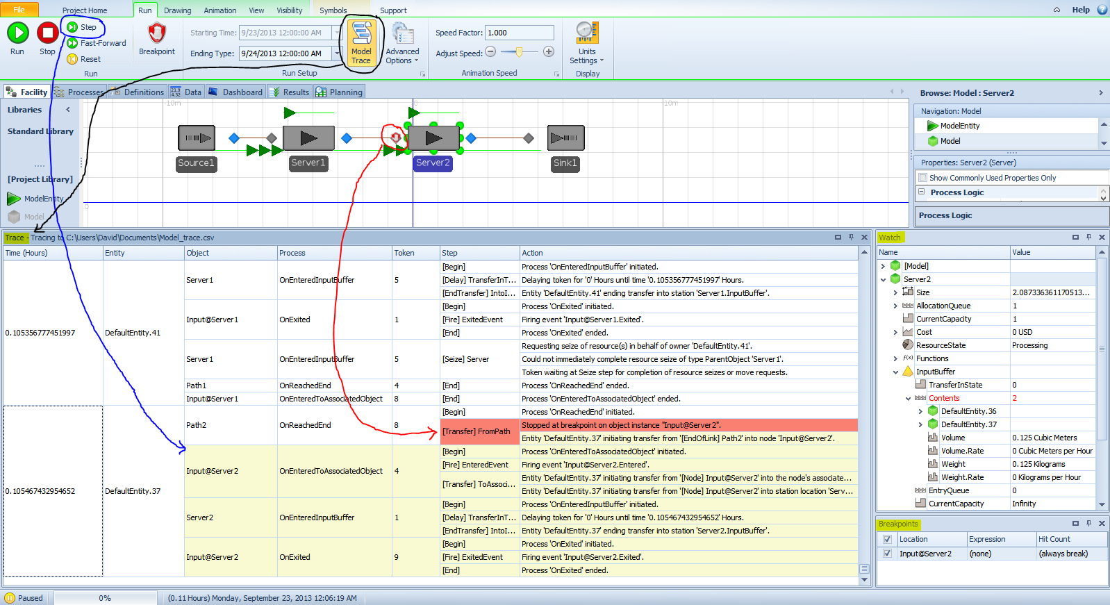
Figure 4.38: Using trace, watch, and break windows in custom layout.

In the default arrangement, these debugging windows display as multiple tabs on the same window. You can drag and drop the individual windows to reproduce the window arrangement in Figure 4.38, or any window arrangement that meets your needs as discussed in Section 4.1.8. Since these windows can be repositioned even on other screens, sometimes you might lose track of a window. In this case press the Reset button found on the Project Home ribbon and it will reset those window positions back to their default layout.

4.10 Summary

In this chapter we’ve introduced Simio and developed several simple Simio models using the Standard Library and using Simio processes. Along the way, we integrated statistical analysis of simulation output, which is just as important as modeling in actual simulation projects, via topics like replications, run length, warm-up, model verification, and the analysis capabilities made possible by the powerful SMORE plots. We started out with an abstract queueing model, and added some interesting context in order to model a somewhat realistic queueing system. In the process, we also discussed use of Simio Paths to model entity movement and basics of animation with Simio. All of these Simio and simulation-related topics will be covered in more detail in the subsequent chapters, with more interesting models.

4.11 Problems

1. Create a model similar to Model 4-1 except use an arrival rate, \(\lambda\), of 120 entities per hour and a service rate, \(\mu\), of 190 entities per hour. Run your model for 100 hours and report the number of entities that were created, the number that completed service, and the average time entities spend in the system.

2. Develop a queueing model for the Simio model from Problem 1 and compute the exact values for the steady state time entities spend in the system and the expected number of entities processed in 100 hours.

3. Using the model from Problem 1, create an experiment that includes 100 replications. Run the experiment and observe the SMORE plot for the time entities spend in the system. Experiment with the various SMORE plot settings — viewing the histogram, rotating the plot, changing the upper and lower percentile values.

4. If you run the experiment from Problem 3 five (or any number of) times, you will always get the exact same results even though the interarrival and service times are supposed to be random. Why is this?

5. You develop a model of a system. As part of your verification, you also develop some expectation about the results that you should get. When you run the model, however, the results do not match your expectations. What are the three possible explanations for this mismatch?

6. In the context of simulation modeling, what is a replication and how, in general, do you determine how many replications to run for a given model?

7. What is the difference between a steady-state simulation and a terminating simulation?

8. What are the initial transient period and the warm-up period for a steady-state simulation?

9. Replicate the model from Problem 1 using Simio processes (i.e., not using objects from the Standard Library). Compare the run times for this model and the model from Problem 1 for 50 replications of length 100 hours.

10. Run the ATM model (Model 4-3) for 10 replications of length 240 hours (10 days). What are the maximum number of customers in the system and the maximum average number of customers in the system (recall that we mentioned that our model would not consider the physical space in the ATM). Was our assumption reasonable (that we did not need to consider the physical space, that is)?

11. Describe how SMORE plots give a quick view of a system’s risk and the sampling error associated with a run of the model.

12. Animate your model from Problem 1 assuming that you are modeling a cashier at a fast food restaurant — the entities represent customers and the server represents the cashier at the cash register. Use Simio’s standard symbols for your animation.

13. Modify your model from Problem 1 assuming that you are modeling a manufacturing process that involves drilling holes in a steel plate. The drilling machine has capacity for up to 3 parts at a time (\(c=3\) in queueing terms). The arrival rate should be 120 parts per hour and the processing rate should be 50 parts per hour. Use Trimble 3D Warehouse to find appropriate symbols for the entities (steel plates) and the server (a drill press or other hole-making device). Add a label to your animation to show how many parts are being processed as the model runs.

14. Build Simio models to confirm and cross-check the steady-state queueing-theoretic results for the four specific queueing models whose exact steady-state output performance metrics are given in Section 2.3. Remember that your Simio models are initialized empty and idle, and that they produce results that are subject to statistical variation, so design and run Simio Experiments to deal with both of these issues; make your own decisions about things like run length, number of replications, and Warm-up Period, possibly after some trial and error. In each case, first compute numerical values for the queueing-theoretic steady-state output performance metrics \(W_q\), \(W\), \(L_q\), \(L\), and \(\rho\) from the results in Section 2.3, and then compare these with your simulation estimates and confidence intervals. All time units are in minutes, and use minutes as well throughout your Simio models.

    1. \(M/M/1\) queue with arrival rate \(\lambda = 1\) per minute and service rate \(\mu = 1/0.9\) per minute.

    2. \(M/M/4\) queue with arrival rate \(\lambda = 2.4\) per minute and service rate \(\mu = 0.7\) per minute for each of the four individual servers (the same parameters used in the mmc.exe command-line program shown in Figure 2.2).

    3. \(M/G/1\) queue with arrival rate \(\lambda = 1\) per minute and service-time distribution’s being gamma(2.00, 0.45) (shape and scale parameters, respectively). You may need to do some investigation about properties of the gamma distribution, perhaps via some of the web links in Section 6.1.3.

    4. \(G/M/1\) queue with interarrival-time distribution’s being continuous uniform between 1 and 5, and service rate \(\mu = 0.4\) per minute (the same situation shown in Figure 2.3).

15. Build a Simio model to confirm and cross-check the steady-state queueing-theoretic results from your solutions to the \(M/D/1\) queue of Problem 9 in Chapter 2. Remember that your Simio model is initialized empty and idle, and that it produces results that are subject to statistical variation, so design and run a Simio Experiment to deal with both of these issues; make your own decisions about things like run length, number of replications, and Warm-up Period, possibly after some trial and error. For each of the five steady-state queueing metrics, first compute numerical values for the queueing-theoretic steady-state output performance metrics \(W_q\), \(W\), \(L_q\), \(L\), and \(\rho\) from your solutions to Problem 9 in Chapter 2, and then compare these with your simulation estimates and confidence intervals. All time units are in minutes, and use minutes as well throughout your Simio model. Take the arrival rate to be \(\lambda = 1\) per minute, and the service rate to be \(\mu = 1/0.9\) per minute.

16. Repeat Problem 15, except use the \(D/D/1\) queueing model from Problem 10 in Chapter 2.

17. In the processes-based model we developed in Section 4.3, we used the standard Token.TimeCreated token state to determine the time in system. Develop a similar model where you manually mark the arrival time (as illustrated in Figure 4.13 and used that value to record the time in system. Hint: You will need to create a custom token with a state variable to hold the value and use an Assign step to store the current simulation time when the token is created.

References

Banks, J., J. S. Carson II, B. L. Nelson, and D. M. Nicol. 2005. Discrete-Event System Simulation. Fourth. Pearson Prentice Hall, Upper Saddle River, New Jersey.

Law, A. M. 2015. Simulation Modeling and Analysis. Fifth. McGraw-Hill, New York.

Nelson, B. L. 2008. “The MORE Plot: Displaying Measures of Risk & Error from Simulation Output.” Proceedings of the 2008 Winter Simulation Conference, 413–16.

Savage, S. L. 2009. The Flaw of Averages: Why We Underestimate Risk in the Face of Uncertainty. Wiley, Hoboken, New Jersey.

Tukey, J. W. 1977. Exploratory Data Analysis. Addison-Wesley, Reading, Massachusetts.