Simio and Simulation: Modeling, Analysis, Applications - 7th Edition
A Case Studies Using Simio
This chapter includes four “introductory” and two “advanced” case studies involving the development and use of Simio models to analyze systems. These problems are larger in scope and are not as well-defined as the Problems in previous chapters. For the first two cases, we’ve also provided some analysis results based on our sample models. However, unlike the models in previous chapters, we do not provide detailed descriptions of the models themselves.
The first case (Section A.1) describes a manufacturing system with machining, inspection, and cleaning operations, and involves analyzing the current system configuration along with two proposed improvements. The second case (Section A.2) analyzes an amusement park and considers a “Fast-Pass” ticket option and the impact it might have on waiting times. The third case (Section A.3) models a restaurant and asks about the important issues of staffing and capacity. The fourth case (Section A.4) considers a branch office of a bank, with questions about how scheduling and equipment choice affect costs.
The two advanced case studies are intended to represent larger realistic problems that might be encountered in a non-academic setting. In the “real world,” problems are typically not as well-formed, complete, or tidy as they are in typical homework Problems. You often face missing or ambiguous information, tricky situations, and multiple solutions based on problem interpretation. You may expect the same from these cases. As these situations are encountered, you should make and document reasonable assumptions.
Case Study videos suitable for featuring in a class can be found here: https://www.simio.com/solution-series/.
A.1 Machining-Inspection Operation
A.1.1 Problem Description
You’ve been asked to evaluate your company’s current machining and inspection operation (see Figure A.1) and investigate two potential modifications, both of which involve replacing the inspection station and its single worker with an automated inspection process. The goal of the proposed modification is to improve system performance.
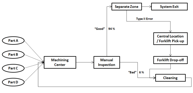
Figure A.1: Machining-inspection operation layout.
In the current system, four different part types arrive to an automated machining center, where they’re processed one part at a time. After completing machining, parts are individually inspected by a human inspector. The inspection process is subject to error — classifying “good” parts as “bad” (type I error) or classifying “bad” parts as “good” (type II error). After inspection, parts classified as “good” are sent to another zone in the plant for further processing, while parts classified as “bad” must be cleaned in an automatic cleaner (with a capacity of one part) and then re-processed by the machining center (using the same processing parameters as “new” parts).
Additional details of the system include:
- Part arrival, machining time, and cleaning time process details are given in Table A.1. All four arrival processes are stationary Poisson processes, and independent of each other.
- All parts go to inspection immediately following machining. The time to inspect a part is independent of the part type and follows an exponential distribution with mean 2 minutes. 6% of inspected parts are found to be “bad” and must be cleaned and then re-processed (this is independent of the number of times a part has been cleaned and re-processed). Parts that fail inspection have priority over the “new” parts in the machining queue after they’re cleaned. It takes 12 minutes to clean each part (the cleaning time is also independent of part type).
- Out of all the parts that are deemed “good” and sent to another zone, 3% are later found to be “bad” (type II error). These parts are put on a pallet in a central location where a forklift will periodically pick up and deliver the pallet to the cleaning machine. These parts are given priority in the automatic cleaner queue. The time between forklift pickups is exponentially distributed with mean 3 hours.
- Out of all the parts that are deemed “bad” and sent to the automatic cleaner, 7% were actually good and did not require cleaning and re-machining (type I error). The per-part cost associated with the unnecessary cleaning and processing is given in Table A.2.
- The machining center and cleaning machine are both subject to random, time-dependent failures. For both machines, the up times follow an exponential distribution with mean 180 minutes, and the repair times follow an exponential distribution with mean 15 minutes. If a part is being processed when either of the machines fails, processing is interrupted but the part is not destroyed.
- The system operates for two shifts per day, six days per week. Each shift is eight hours long and work picks up where it left off at the end of the previous shift (i.e., there’s no startup effect at the beginning of a shift).
| Type | Arrival Rate (parts/hour) | Machining-Time Distribution |
|---|---|---|
| A | 5.0 | tria(2.0, 3.0, 4.0) minutes |
| B | 6.0 | tria(1.5, 2.0, 2.5) minutes |
| C | 7.5 | expo(1.5) minutes |
| D | 5.0 | tria(1.0, 2.0, 3.0) minutes |
| Item | Cost |
|---|---|
| Unnecessary cleaning due to type I error | $5/part |
| Simple robot | $1,200/week each |
| Complex robot | $5,000/week |
| Holding cost per part | $0.75/hour spent in system |
| Inspection worker | $50/hour |
The two scenarios you’ve been asked to evaluate both concern possible automation of the inspection operation:
- Installation and use of four “simple” robots, one for each part type. These robots inspect one part at a time. The probabilities of type I and type II errors are 0.5% and 0.1%, respectively. The time for each “simple” robot to inspect a part is independent of the part type and follows a triangular distribution with parameters (5.5, 6.0, 6.5) minutes.
- Installation and use of one “complex” robot that can inspect all four different part types, but can inspect only one part at a time. The probabilities of type I and type II errors are 0.5% and 0.1% respectively. The time for the “complex” robot to inspect a part is independent of the part type and follows the a triangular distribution with parameters (1.0, 2.0, 2.5) minutes.
Since these robots are manufactured by the same company as the machining center and automatic cleaner, the robots are assumed also to be subject to random failures with the same probability distributions as given above for the machining and cleaning machines. The cost data to be used in your analysis are in Table A.2. Economic analysis for purchasing the robots has already been developed, and the associated costs (purchase price, installation, operation and maintenance, etc.) are given as a single weekly cost in Table A.2.
Develop a Simio simulation to analyze and determine which inspection process your company should use. Your results should include estimates of the following for each scenario:
- Average total cost incurred each week.
- Average numbers of type I and type II errors each week.
- Average total number of parts that finish processing (exit the system) each week.
Using your Simio model, answer the following questions. Your answers should be supported by results and analysis from your simulation experiment(s).
- After looking at the specifications for the robots, the manager has noticed that the average time of inspection for a “simple” robot is much higher than that of the current process. He is nervous that changing the current inspection process might actually decrease overall production (i.e., number of completed parts per week). Will changing the method of inspection change the number of parts that are completed each week? If so, describe how the number of completed parts changes with respect to the current system (i.e., amount of increase/decrease).
- Given the three methods of inspection, which operation do you recommend to minimize costs?
- If you find that one or both of the automatic inspection processes costs the same as, or more than, manual inspection, determine what would enable that inspection process to operate at a weekly cost that’s lower than that with manual inspection. Assume that all costs are fixed and can’t be adjusted.
A.1.2 Sample Model and Results
This section gives the results for a sample model that the authors built. Note that the results depend on a number of assumptions, so your results might not match exactly.The Facility View of the sample model is shown in Figure A.2.
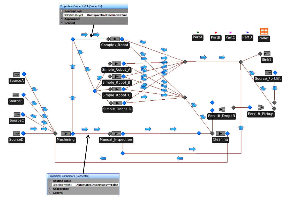
Figure A.2: Facility View of the sample machining-inspection model.
For our experimentation, we used the following controls and parameters:
- Run length: 192 hours
- Warm-up period: 96 hours
- Number of replications: 2,000
- Experiment Controls:
- Automatic Inspection (boolean operator)
- One Inspection Machine (boolean operator)
- Weekly Machine Cost
- Inspection Worker Hours
- Warm-up
Figure A.3 shows how the different controls were used in the Simio Experiment to govern a given scenario’s activity and total cost. We essentially coded all three options into a single model so that we could use Simio’s scenario-comparison capabilities in our analysis. In order to compare the different scenarios in the same experiment, the boolean operators Automatic Inspection and One Inspection Machine were used. When the box associated with a control is checked, the property is given the value of True. The model references these values in the selection-weight property of the connectors before the different inspection processes. Two examples of this are called out in Figure A.2.
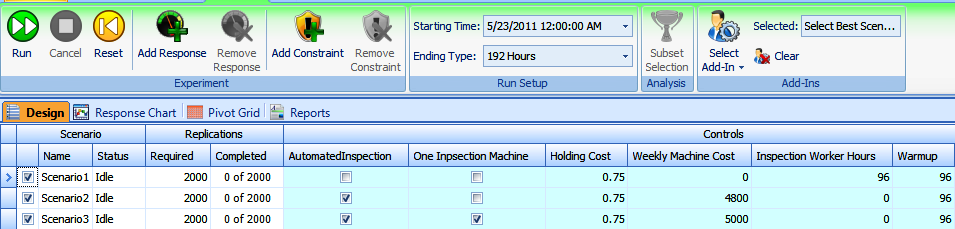
Figure A.3: Snapshot of the machining-inspection Experiment Design.
The expression that we use for the total weekly cost is:
TotalCost = WeeklyMachineCosts + WeeklyHoldingCost.Value + TotalTypeIErrors.Value*5 + InspectionWorkerHours*50
The methods for calculating each of the four sections of the above equation are:
WeeklyMachineCosts: These costs were given in the problem description. The property WeeklyMachineCosts is a standard numeric property that’s controlled in the experiment.
WeeklyHoldingCost.Value: This is the value of the output statistic that references the model state HoldCost. We increment the state HoldCost each time an entity enters the sink (exits the system) using
HoldCost = (TimeNow-ModelEntity.ArrToSys)*0.75 + HoldCostwhich, in essence, calculates the total time the entity spent in the system and multiplies that value by the holding cost given in the problem description. The state is then incremented using this value. Using this method, the output statistic WeeklyHoldingCost will be the sum of the holding costs for all entities.TotalTypeIErrors.Value x 5: The cost of $5 was given in the problem description as the cost associated with a type I error. TotalTypeIErrors is an output statistic that references the model state, TypeIError. This state is incremented when a type I error is committed in the inspection process.
InspectionWorkerHours x 50: The cost of $50 per hour was given in the problem description. The property
InspectionWorkerHoursis a standard numeric property that’s controlled in the experiment.
Using the expression and the experiment parameters listed above, the average weekly cost for each scenario was calculated. These results are shown in Table A.3 (all half widths are of 95% confidence intervals on the expected value). The average weekly totals of type I and type II errors for each inspection process are given in Table A.4. The average total number of parts that finish processing (exit the system) each week can be seen in Table A.5.
| Inspection scenario | Cost | Half width |
|---|---|---|
| Current manual | $7,303.31 | $63.20 |
| Automated: four “simple” robots | $7,268.96 | $58.13 |
| Automated: one “complex” robot | $7,119.54 | $56.37 |
| Inspection scenario | Type I errors [95% CI] | Type II errors [95% CI] |
|---|---|---|
| Current manual | 10.23 [10.09, 10.37] | 69.93 [69.55, 70.31] |
| Automated: four “simple” robots | 1.02 [0.97, 1.06] | 2.26 [2.19, 2.32] |
| Automated: one “complex” robot | 1.04 [1.00, 1.09] | 2.24 [2.17, 2.30] |
| Inspection scenario | Finished parts | Half width |
|---|---|---|
| Current manual | 2,255.29 | 2.21 |
| Automated: four “simple” robots | 2,253.88 | 2.13 |
| Automated: one “complex” robot | 2,255.95 | 2.18 |
A.1.2.1 Answers to Questions
1. Will changing the method of inspection change the number of parts that are completed each week? If so, describe how the number of completed parts changes with respect to the current system (i.e., amount of increase/decrease).
Although the answer to this question could be obtained through simple queueing analysis (for any stable system, flow in equals flow out, so the expected number of parts will simply be the arrival rate times the duration), we can use the results from our simulation experiment to answer this question as well. As seen in the SMORE plot in Figure A.4, it appears that the average total number of parts processed per week does not vary much across the scenarios. To verify that there is no statistically significant difference between the mean number of completed parts per week in scenario 1 (current manual inspection) on the one hand, vs. each of scenario 2 (automated inspection using four “simple” robots) and scenario 3 (automated inspection using one “complex” robot), two different paired \(t\) tests were conducted. The results from these tests are in Figures A.5 and A.6.
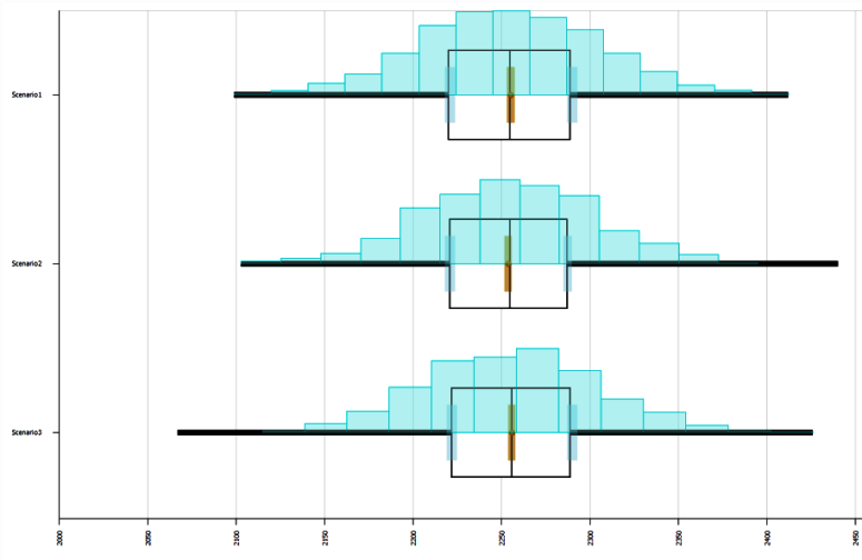
Figure A.4: SMORE plot of the average number of completed parts per week for each scenario.
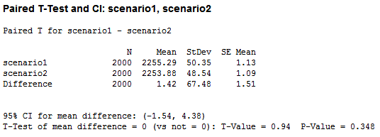
Figure A.5: Minitab results for a paired \(t\) test comparing scenarios 1 and 2.
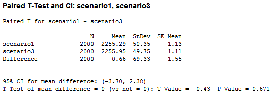
Figure A.6: Minitab results for a paired \(t\) test comparing scenarios 1 and 3.
Since the 95% confidence interval of the mean difference, \([-1.54, 4.38]\), contains zero, we conclude that there is no statistically significant difference between scenarios 1 and 2 with respect to the average numbers of parts processed per week. The same determination can be made from Figure A.6, where scenarios 1 and 3 are compared. Again, there is no statistically significant difference between scenarios 1 and 3 with respect to the average numbers of parts processed per week since the 95% confidence interval of the mean difference, \([-3.70, 2.38]\), contains zero. With this statistical evidence, we can conclude that changing the method of inspection will not significantly change the number of parts completed each week.
Another approach to compare these scenarios involves Simio’s Scenario Subset Selection capability. When the objective functions of the responses are set according to Table A.6, and the “Subset Analysis” is activated, Simio uses a ranking-and-selection procedure to group the response values into subgroups, “Possible Best” and “Reject,” within each response. In the Experiment Window’s Design window, the cells in a Response column will be highlighted brown if they’re considered to be “Rejects,” leaving the “Possible Best” scenarios with their intended coloring. The results obtained through this analysis method are in Figure A.7.
| Response | Objective |
|---|---|
| Total processed | Maximize |
| Type I errors | Minimize |
| Type II errors | Minimize |
| Time in system (TIS) | Minimize |
| Total cost | Minimize |
| Holding cost per week | Minimize |
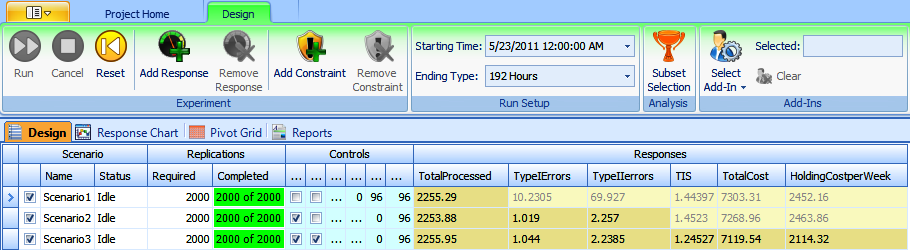
Figure A.7: Results for analysis of several responses using Simio’s Subset Selection.
Simio’s analysis using Scenario Subset Selection gives us the same results as did our paired \(t\) tests. The response, TotalProcessed, for each scenario has not been highlighted brown; therefore, Simio’s Subset Selection has identified each of the three scenarios as a “Possible Best” for maximizing the average weekly number of parts processed. This analysis verifies our expectation that there is no significant difference in the numbers of parts that are processed each week.
2. Given the three methods of inspection, which operation do you recommend to minimize costs?
By examining the SMORE plot shown in Figure A.8, it’s not clear which inspection method would be the least expensive. To determine if there’s any statistically significant difference between the weekly costs for the different scenarios, we again use Simio’s Scenario Subset Selection. Figure A.7 shows that the response values associated with the total cost of scenarios 1 and 2 are both highlighted in brown, indicating a “Reject,” and the response value associated with the total cost of scenario 3 has been identified as a “Possible Best.” Based on this information, and the fact that the overall production does not decrease, we can recommend that the company should change their inspection process to use the one “complex” robot.
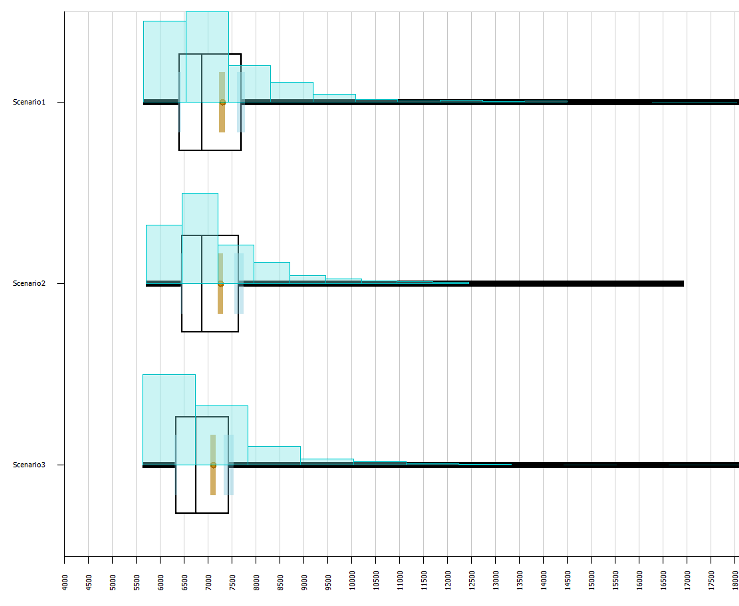
Figure A.8: SMORE plot of the total cost for each scenario.
3. If you find that one or both of the automatic inspection processes costs no less than manual inspection, determine what would enable that inspection process to operate at a weekly cost that’s lower than that with manual inspection. Assume that all costs are fixed and can’t be adjusted.
As discussed above, there is no statistically significant difference between the weekly costs of scenarios 1 and 2. To determine what would lower the costs of this inspection process, we consider the elements that comprise the total cost in equation above. The three costs that are driving scenario 2’s total cost are the machine cost, the cost associated with type I errors, and the holding cost. Since lowering the fixed machine cost is not an option and the type I errors are only costing about $5 per week, it seems that we must lower the holding cost in order to lower the total cost of scenario 2. Since the holding cost is directly related to the amount of time a part spends in the system, reducing the processing time for the four simple machines may seem like a reasonable solution. This hypothesis is also supported by the results in Figure A.7, since the scenario with the lowest total cost also possessed the lowest weekly holding cost and lowest average time that an entity spends in the system. To test this hypothesis, we set up an experiment where we systematically reduced the processing time for the “simple” robots (see Table A.7).
| Scenario | “Simple” robot inspection time |
|---|---|
| Original scenario 1 (manual inspection) | N/A |
| Original scenario 2 | tria(5.5, 6.0, 6.5) |
| Original scenario 3 (automated “complex” inspection) | N/A |
| Scenario 4 | tria(5.4, 5.9, 6.4) |
| Scenario 5 | tria(5.3, 5.8, 6.3) |
| Scenario 6 | tria(5.2, 5.7, 6.2) |
| Scenario 7 | tria(5.1, 5.6, 6.1) |
| Scenario 8 | tria(5.0, 5.5, 6.0) |
As seen in Figure A.9, as the average processing time for the “simple” robots decreases, the total cost decreases as well. As seen in Table A.7, scenarios 4–8 use “simple” robot inspection times with decrements of 0.1 minute. Using the Simio Scenario Subset Selection, we can further analyze the effects of altering the processing times for the “simple” robot. Figure A.10 provides the results of the Subset Selection when the objectives of the Responses are set according to Table A.6.
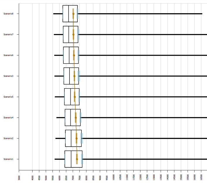
Figure A.9: SMORE plot for the total cost for each of the eight scenarios.
As shown in Figure A.10, the average total cost of scenario 1 is statistically significantly different from that of scenarios 6–8. Therefore, if the manufacturer of the robots can reduce the average processing time by 0.3 minute (through the distribution tria(5.2, 5.7, 6.2)), the inspection operation using the four “simple” robots will yield a lower weekly cost than that of manual inspection. Figure A.10 also shows that there are now four “Possible Best” scenarios: 3, 6, 7, and 8. If we increase the number of replications from 2000 to 2500 for each of these scenarios, and use Scenario Subset Selection, scenario 3 is removed from the subgroup of “Possible Best” (see Figure A.11). The number of completed replications for scenarios 3, 6, 7, and 8 were increased to 2500. With this information, it’s clear that if the manufacturer of the robots can reduce the “simple” robot’s average processing time by 0.3 minute (through the distribution tria(5.2, 5.7, 6.2)), we could recommend the use of the four “simple” robots for part inspections.
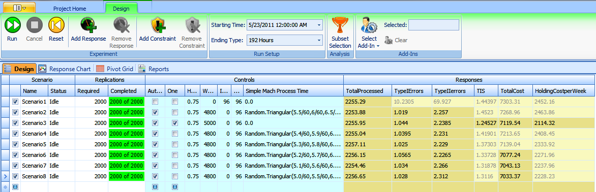
Figure A.10: Results for analysis of several responses for eight scenarios using Simio’s Scenario Subset Selection.
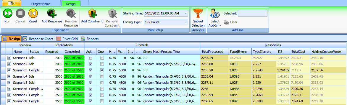
Figure A.11: Previous results with 2500 replications for selected scenarios.
A.2 Amusement Park
A.2.1 Problem Description
An amusement park consists of a roller coaster, a ferris wheel, an arcade, carnival games (one area), concessions, and a bathroom area (see Figure A.12 for the basic layout of the park). The park’s hours are from 10:00 a.m. to 10 p.m. Customers start arriving when the park opens at 10:00 a.m. and stop arriving at 6:00 p.m. Customers arrive according to a non-stationary Poisson process with rate function in Table A.8.
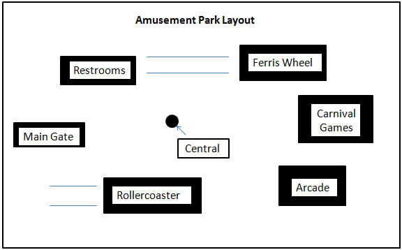
Figure A.12: Amusement-park layout.
| Time interval | Customers per hour |
|---|---|
| 10:00 am - 12:00 pm | 75 |
| 12:00 pm - 2:00 pm | 150 |
| 2:00 pm - 4:00 pm | 100 |
| 4:00 pm - 6:00 pm | 75 |
Once a customer is admitted to the park, he/she has the opportunity to purchase a”Fast Pass,” which allows the customer to have priority at the roller coaster and ferris wheel. The manager of the park has had complaints about wait times from customers since the addition of the Fast Pass and has requested assistance with managing the Fast-Pass process. The manager’s objective is to maximize overall profits of the Fast Pass, subject to the constraints of wait times for Fast-Pass and regular customers.
A.2.1.1 Additional Information
- If there are no Fast Passes handed out for the day, customers typically wait about 20 minutes for rides (this is historical performance information from the current system). While customers are accustomed to waiting at amusement parks, they become extremely dissatisfied after waiting longer than 60 minutes.
- Lines that are “too long” discourage regular customers from entering the respective queue, but Fast-Pass customers have a separate queue and are never discouraged from entering their line. If there are more than 100 people at the roller-coaster line or more than 80 people in the ferris-wheel line, regular customers become discouraged and find something else to do.
- The Fast-Pass customers are willing to wait between 5 and 10 minutes at rides, but become dissatisfied after waiting more than 10 minutes.
- 50% of customers have no interest in going to the arcades.
- 50% of customers will go to the bathroom at most once, and 50% will go at most twice. There are only two bathrooms (capacity of 5 each), currently with an average wait of around 9 minutes over the day.
- Customers do not go to the food area more than once.
- The expected time customers spend in the park varies by customer. Table A.9 gives the probability mass function (PMF) for times spent in the park, which we treat as a discrete random variable with possible values 0.5, 1, 2, 4, or 5 (in hours).
| Hours in park | Probability |
|---|---|
| 0.5 | 0.01 |
| 1.0 | 0.14 |
| 2.0 | 0.25 |
| 4.0 | 0.40 |
| 5.0 | 0.20 |
A.2.1.2 Customer Travel Times and Area Preferences
Customers choose their next destination based on availability and expected wait times. For the bathroom and concession areas, customers are limited to once or twice per visit (as described above). The park has a centrally located “big board” that shows the current expected waiting time for all rides. All customers visit the central area of the amusement park between each area visit to view the big board to help decide where to go next. All areas that are available for the particular customer are equally probable. For example, if the roller coaster has a very long line and the customer has already eaten, and has no interest in the arcade, then the customer has the same probability of going next to the carnival area, bathroom, or ferris wheel. Additionally, when a customer’s time to stay in the park has been surpassed, the path to the exit will become an available option. Customer walk times to and from the central area and all other areas are in Table A.10. The Minimum mentioned in the table represents the minimum time it takes for customers to reach the destination; the Variability represents the mean of an exponentially distributed additional component of the walk time beyond the minimum.
| Area | Minimum | Variability |
|---|---|---|
| Roller coaster | 1 | 1 |
| Ferris wheel | 2 | 1 |
| Carnival games | 2 | 2 |
| Arcade | 3 | 2 |
| Bathroom | 1 | 1 |
| Entrance/exit | 3 | 1 |
A.2.1.3 Ride Areas
The ride-area information is in Table A.11. A car denotes the extra roller coaster car available for loading while the first car is in use. A Ferris-wheel bucket can seat two people at a time.
| Ride | Available | Ride Cap. | Queue Cap. | Ride Time | Load | Unload |
|---|---|---|---|---|---|---|
| Roller coaster | 2 Cars | 20 | 100 | 4 | tria(5,10,13) | 0.5 |
| Ferris wheel | 30 Buckets | 60 | 80 | 10 | 1.2 | 0.5 |
A.2.1.4 Other Areas
The other four areas have unique service times and capacities as shown in Table A.12. The buffer capacity is the maximum number of people who will wait in that area while not being served (e.g., at most five people will wait for an arcade game when all games are being used).
| Area | Time spent in area | Capacity | Buffer capacity |
|---|---|---|---|
| Carnival games | tria(5, 10, 30) | 40 | 40 |
| Arcade | tria(1, 5, 20) | 30 | 5 |
| Bathroom | tria(3, 5, 8) | 10 | 30 |
| Concessions | tria(1, 4, 8) | 4 | 25 |
A.2.1.5 Statistics to Track
- The average and maximum time in queue for both Fast Pass and regular customers for the roller coaster and ferris wheel.
- The average number of Fast Pass and regular customers in the amusement park.
- The average time a Fast Pass and regular customer waits in the queue of a ride.
- The average number of customers waiting and average time waiting at the bathroom.
The manager is interested in the Fast Pass process. Suppose that the park can limit the number of Fast Passes sold (i.e., \(x\%\) of customers in the park will have Fast Passes — the manager is confident that s/he can do this through the pricing of the Fast Pass). What proportion of Fast Passes would you recommend to the manager as a limit before satisfaction is lost and customers become unhappy (i.e., what should \(x\) be)?
A.2.2 Sample Model and Results
This section gives the results for a sample model that the authors built. As with the previous case study, the specific results depend on a number of assumptions, so your results might not match ours exactly. Here are our model specifications:
- Replication run length: 12 hours
- Base time units: minutes
- 100 Replications
Figure A.13 shows the Facility View of our sample model. We expect the waiting times for regular and Fast Pass customers to increase as we increase the number of Fast Pass customers in the park. To test this, we added a property that controls the proportion of Fast Pass customers and created an experiment where we varied this property from 0% to 25% in increments of 1%.
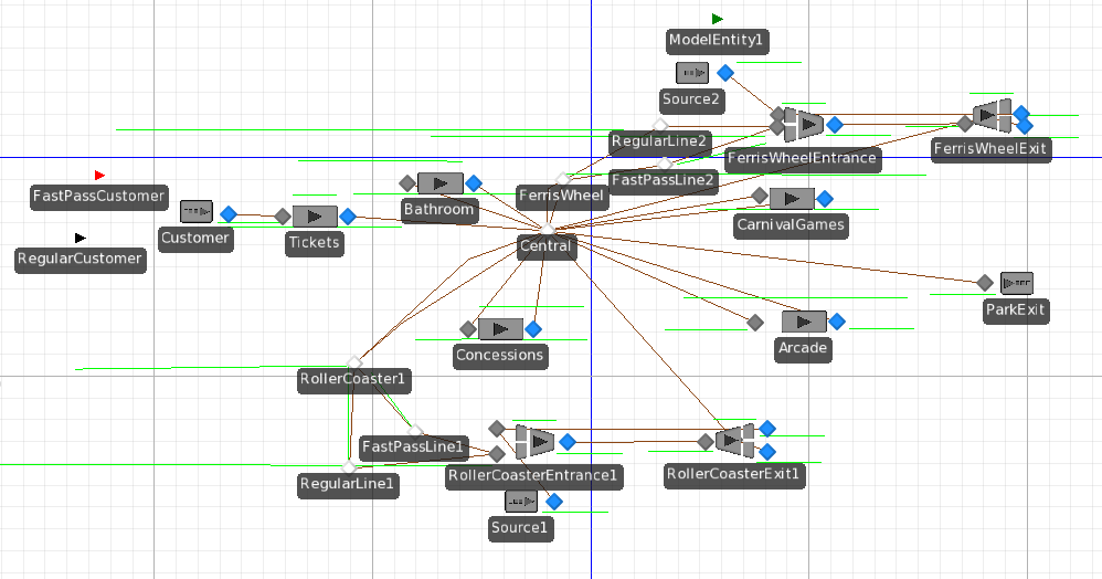
Figure A.13: Sample Simio model for the amusement park case.
Figure A.14 shows the SMORE plot of the response that shows the wait time for regular customers plotted over the percentages of Fast Pass customers. As expected, as the percentage of those who purchase a Fast Pass increases, the wait times increase.
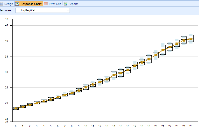
Figure A.14: SMORE plots of average regular customer wait times by percentage of Fast Pass customers.
Similarly, Figure A.15 shows a SMORE plot of the wait time for Fast Pass customers plotted over the percentage of Fast Pass customers. As the percentage of those who purchase a fast pass increases, the wait times also increase.
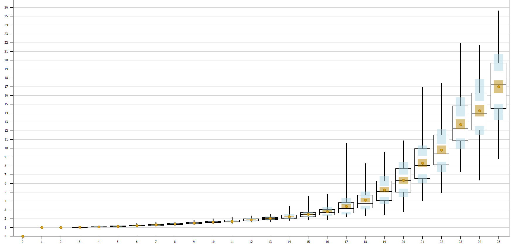
Figure A.15: SMORE plots of average Fast Pass customer wait times by percentage of Fast Pass customers.
In order to determine the “best” proportion of Fast Pass customers, additional cost information for customer waiting would be required. However, the SMORE plots provide relative performance information that would help the manager in making the decision. For example, if 15% of customers have the Fast Pass option, it appears that regular customers would wait between 30 and 35 minutes, and Fast Pass customers would wait approximately 5 minutes. Of course, these estimates are based on a visual inspection of the SMORE plots in Figures A.14 and A.15, and additional, more detailed experimentation would be required to get more precise results.
A.3 Simple Restaurant
A.3.1 Problem Description
The layout of the restaurant is shown in Figure A.16.
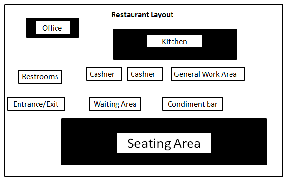
Figure A.16: Restaurant layout.
The restaurant opens at 8:00 a.m., serves breakfast until 11:00 a.m., then serves lunch/dinner until 8:00 p.m. At 8:00 p.m. the doors close, but guests are allowed to stay until they finish their meals.
Customers have the option for dine-in or carry-out (To Go). Historically, 10% of customers order To Go and priority is given to their orders while they’re being made in the kitchen.
A group enters, is greeted, and is given the estimated wait time (if any). If the group is dining in, they decide whether to stay or to leave (balk). If the group elects to stay, the order is placed and food is prepared in the kitchen. A restaurant staff member delivers the order to the waiting group, then the group either leaves (if the group ordered To Go), or sits down at one of the tables. After a group finishes eating, a restaurant staff member clears and cleans the table so others can sit down.
Customers arrive in groups of size 1, 2, 3, or 4, with probabilities 0.10, 0.30, 0.40, and 0.20 respectively, according to a non-stationary Poisson process with the rate function shown in Table A.13.
| Time interval | Groups per hour |
|---|---|
| 8:00 am - 9:00 am | 39 |
| 9:00 am - 10:00 am | 35 |
| 10:00 am - 11:00 am | 48 |
| 11:00 am - 12:00 pm | 44 |
| 12:00 pm - 1:00 pm | 49 |
| 1:00 pm - 2:00 pm | 39 |
| 2:00 pm - 3:00 pm | 26 |
| 3:00 pm - 4:00 pm | 20 |
| 4:00 pm - 5:00 pm | 39 |
| 5:00 pm - 6:00 pm | 48 |
| 6:00 pm - 7:00 pm | 37 |
| 7:00 pm - 8:00 pm | 31 |
The make time for an order depends on the size of the group (e.g. the make time for a group of three will be triple the make time for one order). See Table A.14 for the distribution of service times and the possible number of workers performing the respective tasks. Orders sent to the kitchen are grouped accordingly and delivered together.
| Service | Service-time distribution | Number of workers |
|---|---|---|
| Taking orders | exponential(mean 0.5) | 1-2 |
| Making orders | tria(2, 5, 9) | 5-10 |
| Cleaning tables | exponential(mean 0.5) | 1-2 |
| Distributing | — | 1-3 |
If the expected wait for a table is longer than 60 minutes or there are more than 5 groups waiting for a table, the group will balk. Currently there are 25 tables in the restaurant. The time it takes for groups to eat has a triangular(25, 45, 60) distribution, in minutes.
Currently there are three types of workers: Kitchen workers, general workers, and managers. The kitchen workers prepare and make the orders sent to the kitchen. General workers can work as a cashier (maximum of 2 registers), distribute completed orders, and clean tables. Managers help out with making and distributing orders, but they do not clean tables or work as cashiers. The manager’s priority is making orders in the kitchen. There is at least one manager present at all times. The kitchen gets overcrowded if there are more than ten workers in the kitchen at one time.
Customers waiting longer than 30 minutes (immediately after ordering) become dissatisfied, and food becomes cold eight minutes after being made. Managers are paid $10.00/hour, kitchen workers are paid $7.50/hour, and general workers are paid $6.00/hour. Individual customers spend $9.00 on average.
Current staffing is two managers, eight kitchen workers, and five general workers for a busy day. The owner plans to open a new restaurant with similar expectations and wants to know the following about the current system:
- How many groups balk due to long waits? What is the average wait for a table?
- How many managers, kitchen workers, and general workers should be present each day of the week to minimize labor costs and maintain customer satisfaction (regarding wait times and hot food)? What is the total profit (sales minus labor cost) for the scenario that you chose?
- How many tables are needed to reduce the number of balks due to long waits for a table?
- Since balks occur frequently due to long waits for tables, the restaurant hasn’t experienced its true demand. Create a scenario with the number of tables that you suggested in the previous question. Determine how many workers of each type are needed and the average wait for a table in this system. What is the total profit?
- If the current rate of arrivals increased by 20%, how many tables would you suggest to reduce the number of balks due to long waits for a table?
- If the rate of arrivals decreased by 30%, how many workers of each type would you suggest?
A.4 Small Branch Bank
Consider the following setup and operation of a simple bank branch. The bank branch includes an ATM, a bank of tellers, and a manager. The bank branch is open from 9:00 a.m. to 5:00 p.m., five days a week. Customers arriving after 5:00 p.m. will not be allowed to enter, but the bank will stay open long enough to help all customers in the bank when it closes at 5:00 p.m. A block diagram of the bank is given Figure A.17.
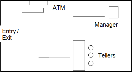
Figure A.17: Bank layout.
Customers arrive in four independent arrival streams, each of which is a nonstationary Poisson process with rate functions being piecewise-constant as given in Table A.15. Arriving customers will either go to the bank of tellers (teller customers), the ATM (ATM customers), or the manager (manager customers) for service. Customers who don’t care whether they get service from a teller or the ATM (teller/ATM customers) will always make their decision based on which line is shortest. If both lines are of equal length, the Teller/ATM customers will always go to the ATM. If the shortest line has more than 4 customers, there is a 70% that customer will leave (balk). All customers who balk are considered to be “unhappy customers.”
| Time period | Teller | ATM | Teller/ATM | Manager |
|---|---|---|---|---|
| 9:00 – 10:00 | 20 | 20 | 30 | 4 |
| 10:00 – 11:30 | 40 | 60 | 50 | 6 |
| 11:30 – 1:30 | 25 | 30 | 40 | 3 |
| 1:30 – 5:00 | 35 | 50 | 40 | 7 |
If there are more than 3 people in the ATM line and fewer than 3 people in the teller line when an ATM customer arrives, there is an 85% chance he/she will switch from being an ATM customer to being a teller customer, and will enter the teller queue, but if the teller queue is occupied by 4 or more people there is an 80% chance that this ATM customer will balk. If there are more than 4 people in the teller line when a teller customer arrives, he/she will balk 90% of the time. There has recently been some economic analysis developed that shows that each “unhappy customer” costs the bank approximately $100 for each occurrence.
While most customers are finished and leave the bank after their respective transaction, 2% of the ATM customers and 10% of the teller customers will need to see the manager after completing service at the ATM or teller. In addition, if a customer spends more than five minutes in the teller queue, there is a 50% chance that he or she will get upset and want to see the manager after completing service at the bank of tellers. If a customer spends more than 15 minutes in the manager queue there is a 70% chance that he or she will get upset. All customers who get upset as a result of waiting time should also considered as “unhappy customers.” Customer travel times between areas of the bank are given in Table A.16 and should be included in your model; assume they’re all deterministic.
| Entry/Exit | ATM | Teller | Manager | |
|---|---|---|---|---|
| Entry/Exit | – | 10 | 15 | 20 |
| ATM | 10 | – | 8 | 5 |
| Teller | 15 | 8 | – | 9 |
| Manager | 20 | 5 | 9 | – |
The ATM can serve one customer at a time and has been known to jam at random times, causing delays for customer transactions. The jam has to be fixed by a “hard reset” of the machine. Recently one of the managers had an intern collect data to determine how often the ATM jams and how long it takes to complete the hard reset. These data can be found in the file ATMdata\_bank.xls in the “students” section of this book’s website (see Appendix C for instructions on how to access this website). Two histograms in reference to these data for the up times (times from the end of a hard reset to the next time the ATM jams) and time required to reset are shown in Figures A.18 and A.19, respectively.
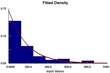
Figure A.18: A histogram of the data gathered for the ATM up times.
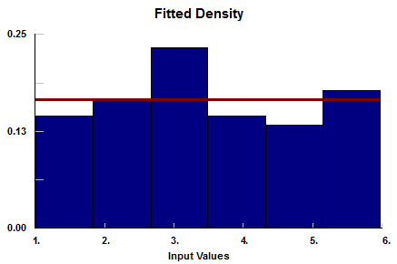
Figure A.19: A histogram of the data gathered for the time to hard-reset a jammed ATM.
The manager can serve one customer at a time and there is one manager on duty at all times. There are two types of tellers, classified as either “experienced” or “inexperienced.” The bank of tellers has a single queue and each teller can serve only one customer at a time. The hourly costs associated with experienced and inexperienced tellers are $65 and $45, respectively. This cost includes the teller’s hourly pay as well as overhead costs (workers compensation, benefits, 401K plans, vacation pay, etc.). Customer service times follow the distributions given in Table A.17.
| Server | Distribution of service time |
|---|---|
| ATM | tria(0.50, 0.83, 1.33) |
| Experienced teller | tria(2, 3, 4) |
| Inexperienced teller | tria(4, 5, 6) |
| Manager | Exponential (mean 5) |
For the manager, the service times are independent of whether the customer has been to the ATM or the teller prior to visiting the manager.
By convention, the bank divides its days into four different time blocks. The mangers of the bank need your help in determining the number of each type of teller that should be scheduled to work during each time block in order to minimize the costs of operating the bank (for analysis purposes, you should be concerned only with the costs that are provided). Because there are only three stations in the teller area, there can be no more than three tellers working during any one time block. Each teller must work the entire time block for which s/he is scheduled:
- Time block 1: 9:00 a.m. – 11:00 a.m.
- Time block 2: 11:00 a.m. – 1:00 p.m.
- Time block 3: 1:00 p.m. – 3:00 p.m.
- Time block 4: 3:00 p.m. – 5:00 p.m.
The managers at the bank have also been considering installation of an additional ATM. The ATM supplier has given the bank two different options for purchasing an ATM. The first option is a brand new machine, and the second option is a reconditioned ATM that was previously used in a larger bank. The supplier has broken the cost down into a daily cost of $500 for the new machine and $350 for the reconditioned machine. % This price is all inclusive and includes installation, operation and maintenance, depreciation, etc…
The reconditioned ATM is assumed to jam and reset at the same rates as the bank’s current ATM machine. Although the new ATM machine is assumed to jam just as often as the current one, it has been enhanced with a faster processor that performs automatic resets in 20 seconds. With this information, the bank management wants your recommendation on whether to purchase an additional ATM machine, and if so, which one.
Use Simio to model this small branch bank as it’s described above. In addition to your model, provide responses to the following items that were requested by the bank managers. Your recommendations should be based on what minimizes the bank’s operating costs with respect to the cost metrics provided in the problem description (“unhappy-customers” cost, additional ATM cost if applicable, and teller cost). Your responses should be supported by your analysis of the results you obtained through experiments.
- Should the bank purchase an additional ATM machine? If so, should it be new or reconditioned?
- Find the number of each classification of tellers that the bank should schedule for each of the four time blocks given in the problem description (i.e., a daily schedule for the bank of tellers).
- What are the bank’s expected daily operating costs with respect to the cost metrics provided in the problem description?
- What is the expected cost per day associated with “unhappy customers?”
- How often does the ATM machine jam? How long does it take to repair it? (The answers to both of these questions should be accompanied by the method you used to obtain them.)
- On average, how many customers is the bank serving per day? This value should include all customers who enter the bank and are involved in some sort of transaction (this should not include customers who leave immediately after entering the bank as a result of a line’s being too long.)
- What proportion of the total arriving customers are considered to be “unhappy customers?”
A.5 Vacation City Airport
The Vacation City Airport (VCA) is a sizeable international airport located near a popular tourist destination, which causes highly variable arrival rates depending on the season. VCA management has surveyed the airline companies about customer service level (CSL) and observed that they were unsatisfied with their total time in system for Terminal 2. Management wants to increase CSL in a cost-conscious way. More specifically, they are looking for objective analysis to help decide between adding new gates or adding a new runway, as well as determining the appropriate staffing. The key parameters are time in system for small and large aircraft, gate utilizations, and utilization of the workers for each operation.
VCA has two international terminals (see Figure A.20). Terminal 1 has 12 parking gates and 16 lanes. Terminal 2 has 12 gates and 42 lanes.
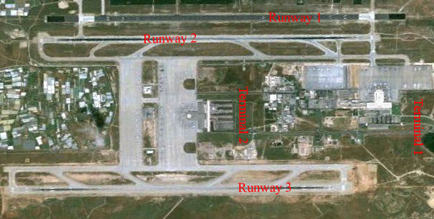
Figure A.20: Vacation City Airport satellite view.
Both terminals are fed by the same three runways, each with different arrival rates. Once an aircraft has landed through one of these runways, it is immediately directed to connecting taxiways to reach the terminal. The aircraft can be directed to parking lanes and gates according to their density. Once parked, it requires several services such as luggage unloading and passenger unloading (which run concurrently), cleaning, fueling, and catering (which run sequentially), and luggage loading and passenger loading (which run concurrently). Each of these service teams has different resources available. Once all services are done, the plane is directed to one of the outbound runways through appropriate taxiways for its take off. The process is summarized in Figure A.21.
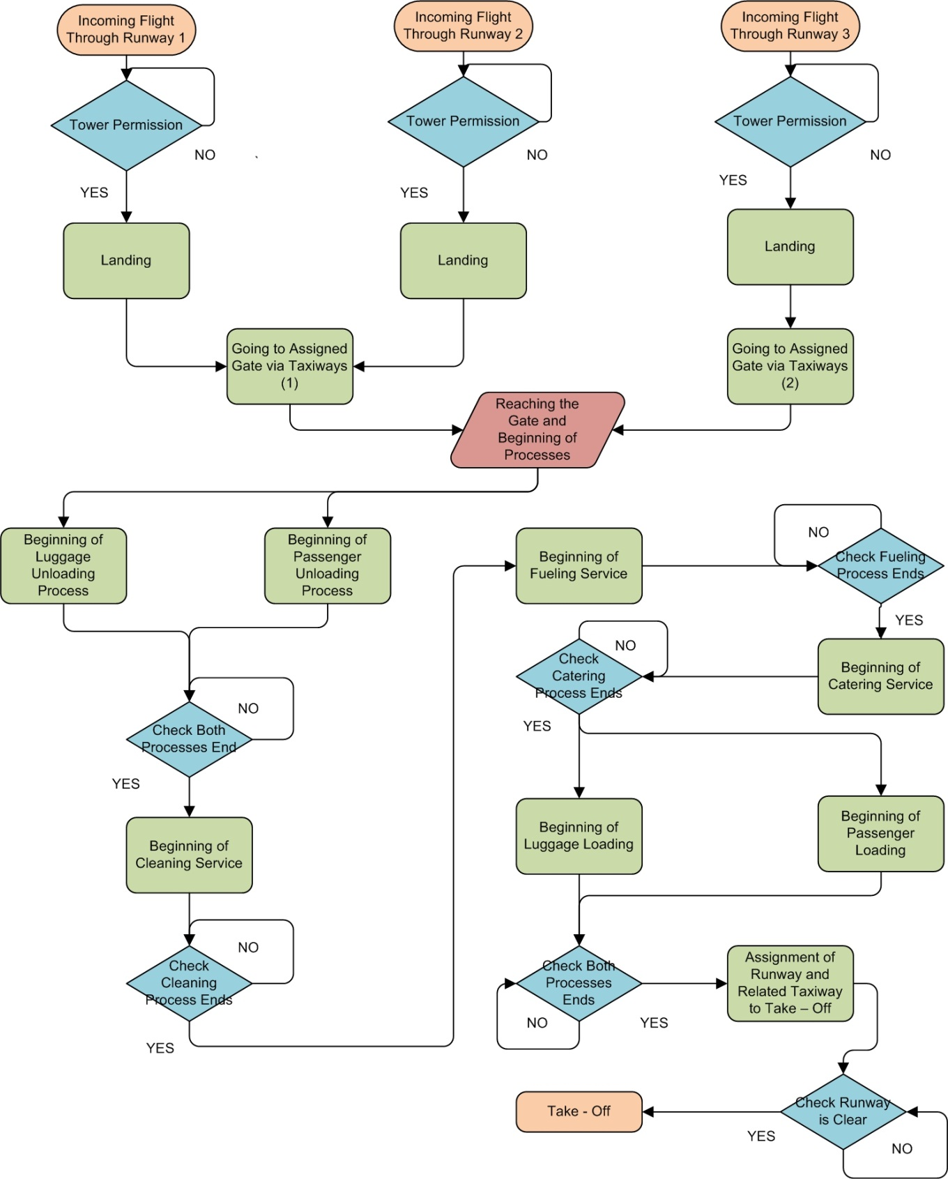
Figure A.21: VCA operation flow chart of existing system.
Table A.18 indicates the team sizes and number of teams available in the existing system.
| Process | Workers per Team | Current Number of Terminal 2 Teams |
|---|---|---|
| Luggage | 2 | 6 |
| Passenger (Unloading, Loading) | 1 | 4 |
| Cleaning | 2 | 2 |
| Fueling | 1 | 2 |
| Catering | 2 | 1 |
Plane arrivals depend on the time of day (see Table A.19). The arrival rate reaches its maximum in the middle of the day. Airport management has categorized aircraft into two groups: large aircraft (at least 120 seats) and small aircraft (fewer than 120 seats). All gates are sized to handle both large and small aircraft. For the planning period in question, the percentage of the above arrivals handled by Terminal 2 are 20% for runway 1, 20% for runway 2 and 30% for runway 3. The balance of the flights are handled by Terminal 1.
| Time | Runway 1 | Runway 2 | Runway 3 |
|---|---|---|---|
| 24 - 1 | 2 | 5 | 3 |
| 1 - 2 | 3 | 6 | 2 |
| 2 - 3 | 1 | 2 | 2 |
| 3 - 4 | 3 | 1 | 1 |
| 4 - 5 | 3 | 3 | 2 |
| 5 - 6 | 2 | 2 | 3 |
| 6 - 7 | 4 | 4 | 4 |
| 7 - 8 | 7 | 6 | 6 |
| 8 - 9 | 9 | 8 | 8 |
| 9 - 10 | 4 | 7 | 5 |
| 10 - 11 | 8 | 6 | 7 |
| 11 - 12 | 6 | 10 | 8 |
| 12 - 13 | 9 | 11 | 11 |
| 13 - 14 | 9 | 10 | 10 |
| 14 - 15 | 12 | 8 | 9 |
| 15 - 16 | 7 | 8 | 7 |
| 16 - 17 | 5 | 8 | 6 |
| 17 - 18 | 5 | 5 | 3 |
| 18 - 19 | 4 | 9 | 7 |
| 19 - 20 | 9 | 6 | 6 |
| 20 - 21 | 7 | 4 | 5 |
| 21 - 22 | 11 | 10 | 9 |
| 22 - 23 | 7 | 8 | 8 |
| 23 - 24 | 6 | 5 | 4 |
The cost of a new 11,000 foot runway is $2,200 per linear foot. The cost of a new 21,000 square foot gate is $28 per square foot. The fully-burdened hourly cost (including associated equipment) of each team is indicated in Table A.20.
| Process | Rate per Team |
|---|---|
| Luggage | $142 |
| Passenger (Unloading, Loading) | $40 |
| Cleaning | $108 |
| Fueling | $150 |
| Catering | $145 |
Acknowledgments: Vacation City Airport is based on a project by Hazal Karaman and Cagatay Mekiker to solve problems for an actual airport. This project was completed as a major part of a graduate-level introductory simulation course at the University of Pittsburgh.
A.6 Simply The Best Hospital
Simply The Best Hospital (STBH) is a rather large hospital that is adopting a pod configuration of its emergency department (ED). A pod is an enclosed area consisting of seven rooms with staff assigned to that pod. They are planning to have six pods, each staffed by one or two nurses. STBH management wants an evaluation of two things:
- What staffing level is required for each pod to ensure that patients don’t have to wait extended periods before being given a room, while not under-utilizing the nurses?
- How much time will it take for a blood test from the time that is ordered until it reaches the lab? The time to carry out the blood test must be kept under fifteen minutes (a policy specific to STBH).
The ED at STBH has two entrances (see Figure A.22).
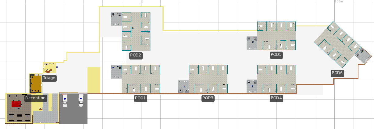
Figure A.22: STBH facility layout.
One entrance is for patients who walk into the ED, and the other entrance is for patients who are brought in by ambulance. Patients who walk in have to go first to the registration desk, where they fill out a form. They then have to go to a triage area where they are diagnosed by a nurse and assigned an acuity. Acuity indicates problem severity (1–5, with 5 being the most serious). When assigned an acuity, the triage nurse enters the patient information into a computer system that assigns every patient to a nurse depending on their availability (if the pod is open, and if they are not busy working with another patient). Then the triage nurse leaves the patient in the corridor for the pod’s nurse to pick up and take him or her to the entrance of a pod that’s open and has a free room. The nurse from the pod then comes to the entrance and takes the patient to his or her room. Here the nurse helps the patient settle into the room, and sets up the necessary equipment. Once the patient has been set up, a doctor comes into the room and may order a blood test for the patient. This happens 75% of the time. When free, the nurse draws blood from the patient, labels it with the patient’s name, and then takes it to the hospital unit cleric (HUC). The HUC takes the blood and labels it with the necessary tests to be done, and then sends it to the lab via a chute. The processing time at the HUC’s desk has a triangular (3, 4, 5) distribution (in minutes).
The file STBH\_ArrivalData.xls in the student area of the textbook web site (see Appendix C) contains arrival data by patient acuity level. From past data, it appears that 80% of acuity 4 patients and 95% of acuity 5 patients arrive by ambulance; all other patients arrive as walk-ins. Processing-time data (assumed to be triangularly distributed with the given minima, modes, and maxima, in minutes) are in Table A.21.
| Patient Acuity | Registration Time | Triage Time | Time in Room |
|---|---|---|---|
| 1 | 3, 5, 8 | 4, 5, 7 | 15, 85, 125 |
| 2 | 3, 5, 8 | 4, 5, 7 | 20, 101, 135 |
| 3 | 3, 5, 8 | 4, 5, 7 | 35, 150, 210 |
| 4 | 1, 2, 4 | 1.5, 2, 4 | 65, 205, 350 |
| 5 | 1, 2, 4 | 1.5, 2, 4 | 90, 500, 800 |
Patients in triage have their blood pressure and temperature taken, and their general complaints are noted. Patients complaining of serious illnesses have expedited triage times, and are taken to the rooms for treatment as soon as possible. Allocation of rooms to patients uses the following strategy: First send incoming patients to pod 1, and when it’s full (all seven rooms are occupied), the next patient will be sent to pod 2 until it fills up, and so on. In the meantime, if a patient has been discharged from pod 1, the next patient to enter the system will be taken to pod 1. This is done so that the minimum numbers of pods are open at any given time, which helps the hospital control costs and staffing. Patients leaving the ED are considered to have left the ED, regardless of whether they leave the hospital.
The key measures that STBH management are looking for are:
- ATWA: Average time in waiting area (average across all types of patients entering the system via walk in).
- NBT: Number of blood tests conducted.
- ATB: Average time for blood test.
- A1TS, … , A5TS: Time in system for each of the 5 acuity levels.
STBH management is particularly interested in six scenarios (other scenarios may also be evaluated):
- Model a day when the staffing of the hospital is lower than the usual level (10 nurses instead of 12), and there happens to be a mass accident like a train or plane crash so about 54 patients of acuity 4 and 5 are brought to the ED.
- Model a period when all the nurses are present but we have roughly 72 more patients of acuities 1, 2, and 3 entering the system during a period of two and a half days. This scenario could be one where a minor epidemic occurs and many people have sore throats, headaches, or upset stomachs.
- Compare a regular week to one where the staffing is low (one nurse per pod) and where the number of patients coming into the hospital is also lower than the norm (200 fewer patients for the week).
- Compare the normal running of the ED in a week where the service times for all the patients increase by 10% throughout.
- Model a weekend (after a normal week) with staffing levels of one nurse per pod.
- Model a period where there is a virus and the ED has 120 patients of acuity 1 and 2 enter over three days. Assume a staffing level that is lower than normal, i.e., there are three pods with two nurses each and the remaining three pods have only one nurse each. Since this involves a virus, assume that 90% of the patients will have blood tests.
Acknowledgments: Simply The Best Hospital is based on a project by Karun Alaganan and Daniel Marquez to solve problems for an actual hospital. This project was completed as a major part of a graduate-level introductory simulation course at the University of Pittsburgh.