Simio and Simulation: Modeling, Analysis, Applications - 7th Edition
Chapter 5 Intermediate Modeling With Simio
The goal of this chapter is to build on the basic Simio modeling and analysis concepts presented in Chapter 4 so that we can start developing and experimenting with models of more realistic systems. We’ll start by discussing a bit more about how Simio works and its general framework. Then we’ll continue with the single-server queueing models developed in the previous chapter and will successively add additional features, including modeling multiple processes, conditional branching and merging, etc. As we develop these models, we’ll continue to introduce and use new Simio features. We’ll also resume our investigation of how to set up and analyze sound statistical simulation experiments, this time by considering the common goal of comparing multiple alternative scenarios. By the end of this chapter, you should have a good understanding of how to model and analyze systems of intermediate complexity with Simio.
5.1 Simio Framework
We’ve touched on quite a few Simio-specific concepts so far. In this section we’ll provide additional detail on many of those concepts, as well as fill in some missing pieces that you’ll need to know in coming sections. While parts of this section might seem a bit detailed (especially to the non-programmers in the audience), we’ll hopefully connect the dots later in this chapter and through the remainder of the book.
5.1.1 Introduction to Objects
In the computer-programming world many professionals believe that object-oriented programming (OOP) is the de facto standard for modern software development — common languages such as C++, Java, and C# all support an object-oriented approach. Discrete-event simulation (DES) is moving down the same path. Many DES products are being developed using OOP but, more important to simulationists, a few also bring the benefits of true objects to the simulation model-building process. Simio, AnyLogic, Flexsim, and Plant Simulation are four popular DES products that provide a true OOP toolkit to modelers.
You might wonder why you should care. For many of the same reasons that OOP has revolutionized the software-development industry, it is revolutionizing the simulation industry. The use of objects allows you to reduce large problems to smaller, more manageable problems. Objects help improve your models’ reliability, robustness, reusability, extensibility, and maintainability. As a result, overall modeling flexibility and power are dramatically improved, and in some cases the modeling expertise required is lower.
In the rest of this section we will explore what Simio objects are and some important terminology. Then we will continue by discussing Simio object characteristics in some detail. While some of this may seem foreign if this is your first exposure to using objects, command of this material is important to understanding and effectively using the object-oriented paradigm.
5.1.1.1 What is an Object?
Simio employs an object approach to modeling, whereby models are built by combining objects that represent the physical components of the systems. An object is a self-contained modeling construct that defines that construct’s characteristics, data, behavior, user interface, and animation. Objects are the most common constructs used to build models. You’ve already used objects each time you built a model using the Standard Library — the general-purpose set of objects that comes standard with Simio. Models 5-1, 5-3, and 5-4 demonstrated the use of the Source, Server, Sink, Connector, and Path objects from Simio’s Standard Library.
An object has its own custom behavior that responds to events in the system as defined by its internal model. For example, a production-line model is built by placing objects that represent machines, conveyors, forklift trucks, and aisles, while a hospital might be modeled using objects that represent staff, patient rooms, beds, treatment devices, and operating rooms. In addition to building your models using the Standard Object Library objects, you can also build your own libraries of objects that are customized for specific application areas. And as you’ll see shortly, you can modify and extend the Standard Library object behavior using process logic. The methods for building your own objects will be discussed in Chapter 11.
5.1.1.2 Object Terminology
So far we’ve used the word “object” somewhat casually. Let’s add a little more precision to our object-related terminology, starting with the three tiers of Simio Object Hierarchy:
An Object Definition defines how an object looks, behaves, and interacts with other objects. It consists of its properties, states, events, external view, and logic. An object definition may be part of your project or part of a library.
ServerandModelEntityare examples of Object Definitions. To edit an object definition, you must first select that object in the Navigation window, then all of the other model windows (e.g., the Processes and Definitions window) will correspond to that object.An Object Instance is created when you drag (or instantiate) an object into your model. An Object Instance includes the property values and may define one or more symbols, but refers back to the corresponding object definition for all the other aspects of the object definition. An Object Instance exists only in your model, but you can have many instances corresponding to a single Object Definition.
Server1,ATM1,DefaultEntity, andATMCustomerare all examples of object instances. To edit an object instance you must select that object instance in a facility view - then you can change its property values and animation.An Object Runspace (also referred to as an Object Realization) is a third tier of objects that holds the current value of an object’s states. Each has a unique ID and may reference a changeable symbol. Object Runspaces are created when you start a run, and in some cases can be dynamically created and destroyed during a run. All Object Instances are destroyed when a run ends. A state in the Runspace for a dynamic object (e.g., an entity) may be referenced using the terminology
InstanceName[InstanceID].StateName. For exampleLiftTruck[2].Prioritywould reference the priority state of the second LiftTruck.
The three tiers of an Entity object are illustrated in Figure 5.1. We have a single entity definition, in this case a person. The entity instances are placed in the model, in this case an Adult person and a Child person. When the model is run, we might create many Adult and Child Runspaces that hold the states of the dynamic entities that are created. We elaborate further on the Simio Object structure in Section 11.1 and, in particular, Figure 11.1.
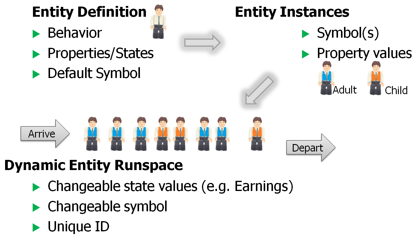
Figure 5.1: The three tiers of an entity object.
We’d be remiss not to mention three other terms that are frequently used when we’re discussing objects:
- A Model is another name to describe an Object Definition. When you’re building a model of your system or subsystem, you’re building an object, and vice-versa. We tend to use the word Object when describing a component (such as the Server object), and use the word Model when referring to the highest-level object (such as the name
Model_04_03on Model 4-3 from the previous chapter). But since even the highest-level object can later be used as a component in some other model, there’s really little difference. - A Project is a collection of Object Definitions (or Models). Most often the objects in a project are related by being designed to work together or to work hierarchically. The file extension SPFX stands for Simio Project File. Because it’s common to think of a project as “building a model,” we often refer to “the model” as a short-hand way of referring what is technically “the project.” Even our example projects are named in this fashion (e.g., Model 5-1) but we trust that you’ll understand.
- A Library is a collection of Object Definitions, or in fact, just another name for a Project. Any Project file can be loaded as a Library using the Load Library button on the Project Home ribbon.
These are key Simio concepts to understand for both using existing Simio objects as well as building your own custom objects. In the next several chapters, we’ll be using existing Simio objects to construct models, and in Chapter 11 we’ll cover the building of custom Simio objects. Technically, when we build a model, we’re already developing a custom Simio object definition, but we’ll refer to these objects as simply models. If you’re new to object-oriented approaches, the fact that a model is an object definition probably seems a bit strange, but hopefully once you gain some experience with Simio, it will begin to make sense.
5.1.1.3 Object Characteristics
As discussed above, an object is defined by its properties, states, events, external view, and logic. Let’s discuss each in more detail.
Properties are input values that can be specified when you place (or instantiate) an object into your model. For example, an object representing a server might have a property that specifies the service time. When you place the server object into your facility model, you would also specify this property value. In Model 5-1, we used the Source object’s Interarrival Time property to specify the interarrival-time distribution and the Server’s Processing Time property to specify the server-processing-time distribution to form an M/M/1 queueing system.
States are dynamic values that may change as the model executes. For example, the busy and idle status of a server object could be maintained by a state variable named Status that’s changed by the object each time it starts or ends service on a customer. In Model 4-2, we defined and used the model state WIP to track the number of entities in the system. When an entity arrives to the system, we increment the WIP state and when and entity departs, we decrement the WIP state. So, at any point in simulated time a specific state provides one component of the overall object’s state. For example, in our single-server queueing system, the system state would be composed of the number of entities in the system (specified by the WIP model state) and the arrival time of each entity in the system (specified by the Entity.TimeCreated entity states).
Events are things that the object may “fire” at selected times. We first discussed the concept of dynamic-simulation events in Section 3.3.1. In our single-server queueing model, we defined entity arrival and service-completion events. In Simio, events are associated with objects. For example, a server object might have an event fire each time the server completes processing of a customer, or an oil-tank object might fire an event whenever it reaches full or empty. Events are useful for informing other objects that something important has happened and for incorporating custom logic.
The External View of an object is the 2D/3D graphical representation of the object. This is what you’ll see when it’s placed in your facility model. So, for example, when you use objects from the Standard Library, you’re seeing the objects’ external views when you add them to your model.
An object’s Logic defines how the object responds to specific events that may occur. For example, a server object may specify what actions take place when a customer arrives to the server. This logic gives the object its unique behavior.
One of the powerful features of Simio is that whenever you build a model of a system, you can turn that model into an object definition by simply adding some input properties and an external view. Your model can then be placed as a sub-model within a higher-level model. Hence, hierarchical modeling is very natural in Simio. We’ll expand on this in Chapter 11.
5.1.2 Properties and States
We briefly mentioned properties and states above, but because you’ll likely be using them a great deal, they deserve some additional discussion.
5.1.2.1 Properties
Properties are defined within an object (see Figure 5.2) to collect information from the user to customize that object’s behavior (note that in this context, the term User refers to the person who instantiates the object and specifies its property values. In the case of Standard Library objects, you are the user of the objects created by Simio LLC employees. But you will learn in Chapter 11 that you can create your own objects and that the user of those objects may be someone other than yourself).
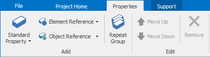
Figure 5.2: Properties ribbon on the Properties view of the Definitions window.
To create or view the properties for an object you must select the object in the Navigation window (not the Facility window), then select the Definitions tab and the Properties item. Properties specific to this object (if any) will appear at the top of this window; properties that are inherited from another object appear in an expandable area just below the other properties.
Properties can be of many different types including:
- Standard: Integer, Real, Expression, Boolean, DateTime, String, …
- Element: Station, Network, Material, TallyStatistic, …
- Object: Entity, Transporter, or other generic or specific object reference
- Repeat Group: A repeating set of any of the above
Tip: When you create a new property it will show up in the object’s Property Window. Sometimes a new property will appear to get “lost.” Make sure that you’re looking in the properties window of the same object to which you added the property (e.g., if you add a property to the ModelEntity object, don’t expect to see it appear on the Model object or a Server object). And if you haven’t given the property a category, by default it will show up in the General category.
Properties can’t change definition during a run. For example, if the user defined the value of 5.3 for a ProcessTime property, it will always return 5.3 and it can’t be changed without stopping the run. However, some property definitions can contain random variables and dynamic states that could return different values even though the definition remains constant. For example, in Model 4-3, we used Random.Triangular(0.25, 1, 1.75) as the Process Time property for the Server object. In this case, the property value itself doesn’t change throughout the model run (it’s always the triangular distribution with parameters 0.25, 1, and 1.75), but an individual sample from the specified distribution is returned from each entity visit to the object. Similarly, we could set a property definition using the name of a state that changes over the model run so that each time the property is referenced, it returns the current value of the state.
The value of a property is unique to each object instance (e.g., the copy of the object that’s placed into the facility window). So for example, you could place three instances of ModelEntity (let’s call them PartA, PartB, and PartC) in your model by dragging three copies of the ModelEntity object from the Project Library onto the Facility view. Each of these will have a property named Initial Desired Speed but each one could have a different value of that property (e.g., The Initial Desired Speed of PartA doesn’t necessarily equal that of PartB). However because properties can’t change their values during a run, those property values are efficiently stored once, with the instance, regardless of how many dynamic entities (Runspaces) are created as the model runs.
5.1.2.2 States
States are defined within an object (see Figure 5.3) to hold the value of something that might change while a model is running. (Note: Since state values can change, they are often referred to as state variables and you should consider the terms state and state variables synonymous in this context.) There are two categories of states: Discrete and Continuous. A Discrete State (or discrete-change state) may change via an assignment only at discrete points in time (e.g., it may change at time 1.2457, then change again at time 100.2). A Continuous State (or continuous-change state) will change continuously and automatically when it’s rate or acceleration is non-zero.
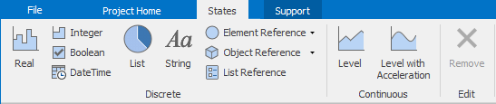
Figure 5.3: States ribbon on the States view of the Definitions window.
States can be one of several types, including:
- Real: A discrete state that may take on any numeric value.
- Integer: A discrete state that may take on only integer (whole) numbers.
- Boolean: A discrete state that may take on only a value of True (1) or False (0).
- DateTime: A discrete state that may be assigned a value in a DateTime format.
- List: An integer value corresponding to one of several entries in a string list (discussed in Section 7.5), often used with statistics and animation.
- String: A discrete state that may be assigned a string value (e.g., “Hello”) and may be manipulated using the String Expression functions such as String.Length.
- Element Reference: A discrete state that may be assigned an element reference value (e.g., indicates an element such as a TallyStatistic or a Material).
- Object Reference: A discrete state that may be assigned an object reference value (e.g., refers to either a generic Object or a specific type of object like an Entity).
- List Reference: A discrete state that may be assigned a list reference value (e.g., refers to list like LocalTrucks or LDTrucks).
- Level: A continuous state that has both a real value (the level) and a rate of change. The state will change continuously when the rate is non-zero. The rate may change only discretely.
- Level with Acceleration: A continuous state that has a real value (the level), a rate of change, and an acceleration. The state may change continuously over time based on the value of a rate of change and acceleration. The rate may change continuously when the acceleration is non-zero. Both the rate and the acceleration may change discretely.
States can be associated with any object. A state on an entity is often thought of as an attribute of that entity. A state on a model can in some ways be thought of as a global variable on that model (e.g., the model state WIP that we used in Model 4-2). But you can have states on other objects to accomplish tasks like recording throughput, costs, or current contents.
States do not appear in the Properties Window, although a Property that’s used to designate the initial value of a State often does appear in the Properties Window. To create or view the states for an object you must select the object in the Navigation window (not the Facility window). For example to add a state to the ModelEntity object, first click on ModelEntity in the navigation window. Once you have the proper object selected, you can select the Definitions tab and the States item. States specific to this object (if any) will appear at the bottom of this window; states that are inherited from another object appear in an expandable area at the top of this window.
The value of a state is unique to each object runspace (i.e. the copies of the object that are dynamically generated during a run) but not unique to the object instance. So for example, an instance of ModelEntity placed in your model (let’s call it PartA) has a property named Initial Desired Speed that is common to all entities of type PartA. But all instances of ModelEntity also have a state named Speed. Because these states can be assigned as they move through the model, each entity created (the dynamic runspace) could have a different value for the state Speed. Hence the value of the Speed state must be stored with the dynamic entity runspaces. Because of the extra memory involved with a state, you should generally use a Property instead of a State unless you need the ability to change values during a run.
5.1.2.3 Editing Object Properties
Whenever you select an object in the Facility window (by clicking on it), the properties of the selected object are displayed for editing in the Properties window in the Browse panel on the right. For example, if you select a Server object, the properties for the Server will be displayed in the Properties window. The properties are organized into categories that can be expanded and collapsed. In the case of the Server in the Standard Library, the Process Logic category is initially expanded, and all others are initially collapsed. Clicking on the triangular symbol on the left side of the property name will expand and collapse a category. Whenever you select a property, a description of the property appears at the bottom of the grid. As discussed above, the properties may be different types such as strings, numbers, selections from a list, and expressions; these are often reflected in the property. For example, the Ranking Rule for the Server is selected from a drop-down list and the Processing Time is specified as an expression. If you type an invalid entry into a property field, the field turns a salmon color and the error window will automatically open at the bottom. If you double-click on the error in the error window it will then automatically take you to the property field where the errors exist. Once you correct the error, the error window will automatically close.
Like much of the OOP world, Simio uses a dot notation for addressing an object’s data. The general form is “xxx.yyy” where yyy is a component of xxx. This is sometimes repeated for several levels when you have sub-components and even sub-sub-components. For example Server1.Capacity.Allocated.Average provides the average allocated capacity for Server1. When you use the Property window this is mostly hidden from you, but you’ll sometimes see this in a drop-down list and you’ll see it as you use the expression builder (briefly discussed earlier in Section 4.5, and more fully below in Section 5.1.7) to construct and edit expressions. As you become more experienced, you may choose to type the dot notation directly rather than using the expression builder.
5.1.2.4 Referenced Properties
Referenced properties are a special application of properties that are generally used in the definition of other properties. For example, you could define a referenced property named PaintingTime and then use PaintingTime as the definition of the ProcessingTime property in a Server object. You can use any existing property in this way, or you can create a new referenced property by right clicking on a property as shown in Figure 5.4.
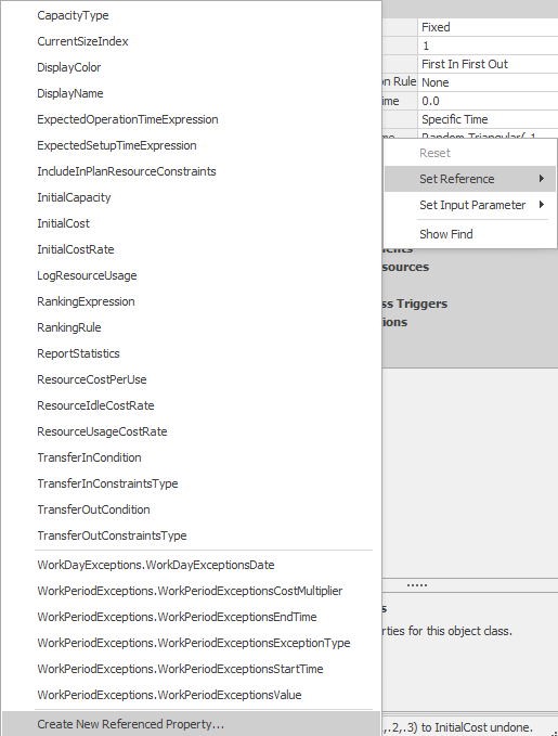
Figure 5.4: Defining a new referenced property.
The are three common reasons to use referenced properties:
- When others are using your model, you might want to make some key parameters (referred to as Controls) easy to find and change. All referenced properties are displayed under a Controls category in the model Properties window (right click on
Modelin the Navigation Window, then selectProperties). You can customize how they’re displayed by changing Default Value, Display Name, Category Name and other aspects in the Definitions - Properties window. - Referenced properties provide an easy way to share properties (e.g., you can specify the value once in a property and use (or reference) it in multiple places). This simplifies experimentation with different property values.
- When you do model experimentation from the Experiment window, referenced properties automatically (unless you set its Visible value to
False) show up as experiment controls. These controls are the items that you may want to vary to define multiple alternative scenarios, such as altering server capacities, which we’ll do in Section 5.5.
Referenced properties are displayed with a green arrow marker when used as property values (see Figure 5.5). When running a model interactively, the values of the controls are set in the model Properties window. When running experiments the values specified for controls in the model properties window are ignored and instead the values that are associated with each scenario in the Experiment Design window are used.
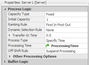
Figure 5.5: Example of using a referenced property.
You’ll see examples of using referenced properties in the models in the current and subsequent chapters.
5.1.2.5 Properties and States Summary
Table 5.1 summarizes some of the differences between properties and states. Note that new users are very often confused about properties and states and, in particular, when one is used rather than the other. Hopefully we can clear up the natural confusion as we develop models with more and more features/components and discuss the use of their properties and states.
| Properties | States | |
|---|---|---|
| Basic Data Types | 22 | 9 |
| Runtime Change | No | Yes |
| Arrays Supported | No | Yes (selected) |
| Where Stored | Object instance | Object runspace |
| Server Example | Processing time | Number processed |
| Entity Example | Initial speed | Current speed |
| Cost Example | Cost per hour | Accrued cost |
| Failure Example | Failure rate | Last failure time |
| Batching Example | Desired batch size | Current batch size |
5.1.3 Tokens and Entities
Many simulation packages have the concept of an Entity — generally the physical “things” like parts and people that move around in a system. But something else is often required to do lower-level logic where an entity may not be involved (like system control logic) or where an entity may actually be doing multiple actions at one time (like waiting for an event during a processing delay). Simio provides Tokens for this extra flexibility.
5.1.3.1 Tokens
A Token is a delegate of an object that executes the steps in a process. Typically, our use of a Token is as a delegate of an Entity, but in fact any object that executes a process will do so using a token as a delegate. A token is created at the beginning of a process and is destroyed at the end of that same process. As the token moves through the process it executes the actions as specified by each step. A single process may have many active tokens moving through it in parallel. And a single object can have many tokens representing it.
A token may also carry its own properties and states. For example, a token might have a state that tracks the number of times the token has passed through a specific point in the logic. In most cases you can simply use the default token in Simio, but if you require a token with its own properties and states you can create one in the Token panel within the Definitions window.
A token carries a reference to both its parent object and its associated object (Figure 5.6). The parent object is an instance of the object in which the process is defined. For example a process defined inside the Server object definition would indicate a server (perhaps Server1) as its parent. The associated object is the related object (separate from the parent object) that triggered this process to execute. For example, a process that’s triggered by an entity arriving to an object will have that entity as the associated object. The process logic can refer to properties, states, and functions of both the parent object and the associated object. Hence, the token could reference the arriving entity to specify the delay time on the Delay step. To reference the associated object it’s necessary to precede the property or state name with the object-class name. For example ModelEntity.TimeCreated would return the value of the TimeCreated function for the associated object of type ModelEntity.
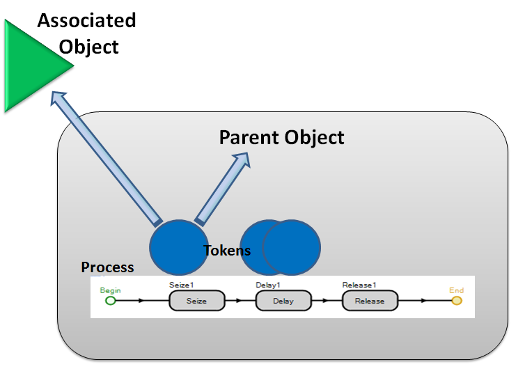
Figure 5.6: Relationships between Tokens, Objects, and Processes.
5.1.3.2 Entities
In Simio, Entities are part of an object model and can have their own intelligent behavior. They can make decisions, reject requests, decide to take a rest, etc. Entities have object definitions just like the other objects in the model. Entity objects can be dynamically created and destroyed, move across a network of links and nodes, move through 3D space, and move into and out of fixed objects.
Examples of entity objects include customers, patients, parts, and work pieces. Entities don’t flow through processes as tokens do. Instead a token is created as a delegate of the entity to execute the process. The movement of entities into and out of objects may trigger an event, which might execute a process. When the process is executed, a Token is created that flows through the steps of a process.
Entities have a physical location within the Facility window and they can reside in either Free Space, in a Station, on a Link, or at a Node (discussed further in Chapter 8). When talking about the location type of an Entity, we’re referring to the location of the Entity’s leading edge. Examples of Stations within Simio are: the parking station of a Node (TransferNode1.ParkingStation), the input buffer of a Server object (Server1.InputBuffer), and the processing station of a Combiner object (Combiner1.Processing).
5.1.4 Processes
In Section 4.3 we built an entire model using nothing but Simio Processes. That was an extreme case for using processes. In fact, every model uses processes because the logic for all objects is specified using processes. We’ll explore that more in Chapter 11. But there’s yet another common use for processes, Add-on Processes, that we’ll explore here.
A process is a set of actions that take place over (simulated) time, which may change the state of the system. In Simio a process is defined as a flowchart using steps that are executed by tokens and may change the state of one or more elements. Referring again to Figure 5.6, you’ll note an object (Parent Object) that contains a process consisting of three steps. The arrows on the first blue token indicate that it has references to both its parent object (e.g., a server) and its associated object (e.g., an entity that initiated this process execution). Note that the other blue tokens in the figure also have similar references.
Processes can be triggered in several ways:
- Simio-defined processes are automatically executed by the Simio engine. For example, the
OnInitializedprocess is executed by Simio for each object on initialization. - Event-triggered processes are user-defined processes that are triggered by an event that fires within the model.
- Add-on processes are incorporated into an object definition to allow the user of that object to insert customized logic into the standard behavior of the object.
For now, let’s just discuss add-on processes a bit more.
5.1.4.1 Add-on Processes
While object-based tools are well-known to provide ease of use, they generally have a major disadvantage. If an object isn’t built to match your application perfectly (and they seldom are), then you either ignore the discrepancy (risking invalid or unusable results), or you change the object or build your own (either of which can be very difficult in some software). To eliminate that problem, Simio introduced the concept of add-on processes. Add-on processes allow you to supplement the standard object logic with additional behavior. Add-on process triggers are part of every standard library object. They exist to provide a high degree of flexibility to modelers.
An add-on process is similar to other processes but is triggered by another object. For example, a Server may have an add-on process that is triggered when an Entity that enters the Server. The object (the Server, in this case) provides a set of Add-on Process Triggers where you can enter the name of a process you want to execute. These processes are often quite simple, but provide incredible flexibility. For example, the Simio Server supports several types of failures, but none of them accounts for the availability of an external resource (e.g., an electrician) before the repair can be started. You could ignore that resource constraint (probably unwise), or create your own object (perhaps tedious), or simply add two processes with one step each to implement this capability. Server has a Repairing add-on process trigger where you’d add a process with a Seize step to obtain an electrician before starting the repair time. Server also has a Repaired add-on process trigger where you’d add a process with a Release step to free the electrician after the repair is complete.
It’s actually quite easy to create these processes. If a process is to be shared or referenced from several different objects, you can go to the Processes tab and create the processes, then complete the logic. But if you’re using a process only once, there’s an even-easier way. We’ll illustrate this by continuing the above example.
Create a new model and place a Source, Server (Server1), and Sink, connected by paths and add a Worker (Worker1) in it. For Server1 change the Failure type to Calendar Time Based, set the Uptime Between Failures to 10 Minutes and set the Time to Repair to 1 Minute. Leave all other properties on all objects at their defaults. At this point we have a simple model using the Standard Library objects that incorporates failures. Now let’s customize the Server behavior to make it use the Worker during repairs.
- In the
Server1properties under Add-on Process Triggers, double clickFailed. Simio will automatically create the add-on process, name it appropriatelyServer1_Failed, categorize it with similar processes (Server1 Add-on Processes category), and then leave you in the process window ready to edit the process. - Drag a
Seizestep into the process. - Complete the Seize step properties: Double click on the Rows property
...and then click theAddbutton to get the resource dialog. SelectWorker1for the object name to seize. Then clickClose. - Back in the Facility window in the
Server1properties, under Add-on Process Triggers, double-clickRepaired. Again note all the automatic behavior that will leave you in the Process window. - Drag a
Releasestep into the Server1_Repaired process. - Complete the Release step properties: Double click on the Rows property
...and then click theAddbutton to get the resource dialog. SelectWorker1for the object name to release. Then clickClose.
Your model should look something like Figure 5.7. If you run the model and look at the interactive results you should see the server failed for 10% of the time and likewise the Worker utilized for a corresponding 10% of the time. Of course, you could make this model more interesting by having the worker do other things when not busy. And a bit later we’ll learn how to move the worker between tasks and consider the worker’s current location in the processing. But for now, you’ve hopefully learned that using add-on processes can provide a lot of flexibility and isn’t all that difficult to do.
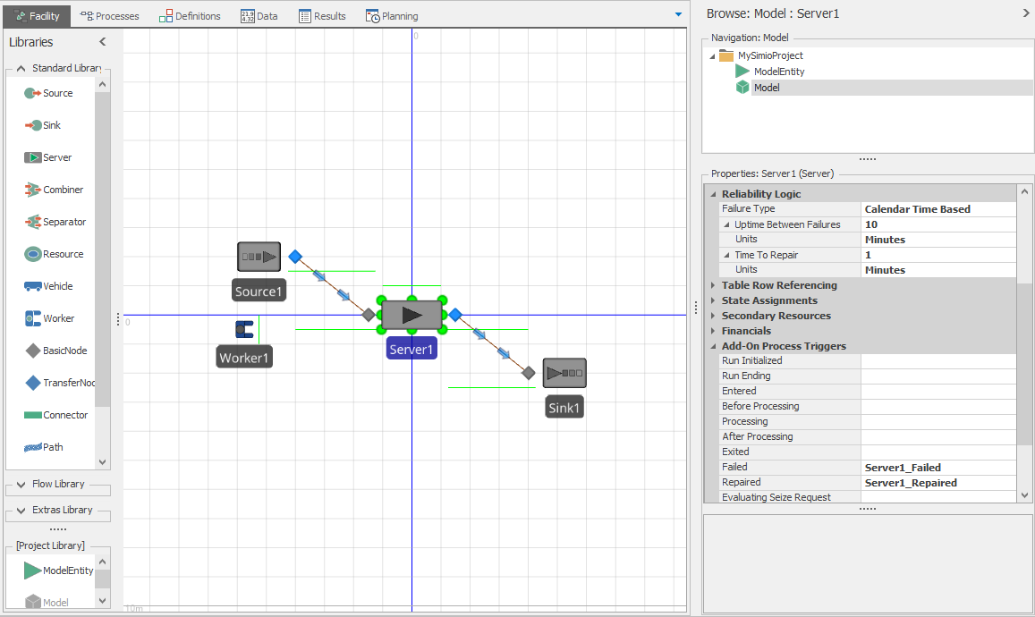
Figure 5.7: Using add-on processes to add a repair resource.
5.1.5 Objects as Resources
In earlier sections we discussed the concept of a resource that represents a constraint in the system. In a previous model (Section 4.3), we specifically used the Resource object from the Standard Library. That Resource object was provided in the library for your convenience, but you’re not limited to that particular object. In fact, any Simio object can be used as a resource. (Note that the object builder may specifically disable that feature by setting the property Resource Object in the object definition to False or hiding some or all of the resource-related properties.).
Being able to be used as a resource includes the capability to:
- Have a capacity constraint.
- Have a queue where tokens wait for capacity to become available.
- Have automatic statistics on scheduled and allocated capacity.
- Intelligently interact with the object attempting to seize it.
Let’s explore each of these in a bit more detail.
Resources have a capacity constraint. The capacity can be 0 (no availability), Infinity (no constraint), or any integer in between. The capacity may also follow a schedule (see Sections 5.3.3 and 7.2). Calendar-based schedules may be defined by selecting the Schedules window under the Data Tab. Here you can configure recurring (such as daily and weekly) schedules and also configure Exceptions to those schedules, such as for holidays or scheduled overtime.
For ultimate flexibility the capacity of a resource can be controlled using process logic and assign steps. This approach allows you to adjust capacity dynamically in reaction to model situations and also to account for any desired transition rules (e.g., what happens to a busy resource when it goes off-shift).
Resources have a queue where tokens wait for capacity to become available. Entities don’t directly take resource capacity. Rather, an entity has a token execute a Seize step inside a process to request that a resource allocate capacity to the entity. All tokens wait in a single allocation queue for a specific resource. If the requested resource isn’t available, the token (and associated entity) must wait. An entity that wants to seize more than one resource, or one of a list of resources, may generate a token waiting in the allocation queue for each resource involved.
The ranking rule for allocation queues may be specified with either static or dynamic ranking. Static ranking rules include First In First Out, Last In First Out, Smallest Value First, and Largest Value First. The latter two rules require a Ranking Expression that’s often a state like Entity.Priority. This expression is evaluated when the queue is entered to determine proper rank. While static ranking is very efficient, dynamic ranking allows superior flexibility when it’s necessary to make a real-time determination of the “best” allocation strategy. Dynamic Ranking examines every waiting entity each time an allocation is attempted. Because dynamic ranking rules must examine every entity each time a decision is made, when the queues are very large it might cause slower execution speed. . In addition to Smallest Value First and Largest Value First, it includes an option for Standard Dispatching Rule under which you will find more sophisticated rules such as Critical Ratio, Least Setup Time, and Campaign Sequence Up. (Note: Campaigns are often used in industries like painting and rolling mills where the exact sequence of processing is very important, like painting successively darker colors or rolling successively narrower strips of steel.). Advanced users also have the capability to create their own dynamic allocation rules (see Chapter 11).
Resources have automatic statistics on scheduled and allocated capacity. These may also be supplemented with state statistics (e.g., Idle, Busy, Blocked, Failed, …). Every resource automatically tracks the average, minimum, and maximum number of capacity units scheduled and capacity units allocated. Many of the standard objects take advantage of the List State feature to track additional state-based detail. For example, the Resource Object tracks the following states:
- Idle - The resource isn’t allocated to any task.
- Busy - The resource has capacity allocated to one or more tasks.
- Failed - The resource is failed and not allocated to any tasks.
- OffShift The resource is off shift and not allocated to any tasks.
- FailedBusy - The resource is failed but allocated to one or more tasks and still assumed “Busy” though failed.
- OffShiftBusy - The resource is off shift but allocated to one or more tasks and still assumed “Busy” though off-shift.
In addition to output statistics, you can also display pie charts of the data in your model or console.
A resource may intelligently interact with the objects attempting to seize it. This feature provides a great deal of modeling latitude. Since objects may have autonomous behavior, this allows the concept of smart resources. In Simio the process of seizing a resource is a negotiation between two objects — both objects must “agree” before the seize occurs. A resource may choose if, and when, it will allow itself to be seized. For example, a resource may prevent itself from being seized close to the end of a shift. Or maybe the resource will choose to remain idle because it’s aware that a higher-priority request will arriving soon. Or it may only consider requests that are in the proximity of its current location.
As you can see, significant intelligence can be built into a resource. Intelligent control of allocations is accomplished by adding logic to the OnEvaluatingAllocation standard process. Some Standard Library objects also have an Evaluating Seize Request add-on process trigger. You’ll learn more about how to take advantage of these in Chapter 11.
5.1.6 Data Scope
The definition of an object can’t know anything about its encompassing object or objects parallel to it in the encompassing object because it can’t know at the time of definition how it will be used, or what object in which it will be placed. For example, if you have a state named DayOfWeek defined on the model, the objects in your model can’t directly reference DayOfWeek. This can be worked around by passing in that item via a property to permit an indirect reference. In fact, that’s exactly what most of the properties in the Standard Library object are for.
Only the information that an object chooses to make public is available outside that object. For example, if you have an object that’s designed to track the calendar and it contains a state named DayOfYear, if DayOfYear is defined as public, then the model and other objects would be able to reference it. If DayOfYear isn’t public then only the calendar object would be able to reference its value.
Add-on processes are at the scope of the encompassing object. This means that Steps in an add-on process can directly reference information in the encompassing model (e.g., the main model), as well as the parent object and the associated object. This also means that data-scope issues are somewhat rare until you get into building your own objects in Chapter 11.
5.1.7 Expression Builder
For expression fields (e.g., Processing Time), Simio provides an expression builder to simplify the process of entering complex expressions; we guided you through a few examples of its use just briefly in Section 4.5, but provide more detail here. When you click in an expression field a small button with a down arrow appears on the right. Clicking on this button opens the expression builder, with a red X and green check mark on the right and a funnel symbol on the left. By default the funnel is “lit up” indicating that a filter has been automatically applied. Although in most models it is unlikely that the list of choices is too small, turning off the filter will expose even more items to choose from.
The expression builder is similar to IntelliSense in the Microsoft family of products and tries to find matching names or keywords as you type using the dot notation discussed in Section 5.1.2.3. Many items in the expression list have required or optional sub-items. Items that have sub-items are identified with a \(>>\) at the right edge, indicating that more choices are available. An item that is not in bold indicates that it’s not yet a valid choice — you can’t stop there and have a valid expression, you must select a sub-item. If the item itself is in bold, that indicates that it is a valid choice — it either has no sub-items or it has only optional sub-items. For example in Figure 5.8 you’ll see that Color, DateTime, DirectDistanceTo, Elements, and Enum are not valid choices, indicated by not being bolded — you’d have to select a sub-item to use one of these. The other three items, all in bold, are valid choices. Of those, the first two (DefaultEntity and Entity) have optional sub-items as indicated by the arrows. The other bold item (False) has no sub-items.
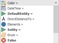
Figure 5.8: Excerpt of expression builder choices.
You can use math operators +, - , * , / and ^ to form expressions, and parentheses as needed to control the order of calculation, like 2*(3+4)^(4/3). Logical expressions can be built using <, <=, >, >=, !=, ==, &&, ||, and !. Logical expressions return a numerical value of 1 when true, and 0 when false. For example 10*(A > 2) returns a value of 10 if A is greater than 2; otherwise it returns a value of 0. Arrays (up to 10 dimensions) are 1-based (i.e., the beginning subscript is 1, not 0) and are indexed with square brackets (e.g., B[2,3,1] indexes into the three dimensional state array named B). Model properties can be referenced by property name. For example if Time1 and Time2 are properties that you’ve added to your model then you can enter an expression such as (Time1 + Time2)/2.
A common use of the expression builder is to enter probability distributions. These are specified in Simio in the format Random.DistributionName(Parameter1, Parameter2, …, ParameterN), where the number and meaning of the parameters are distribution-dependent. For example Random.Uniform(2,4) will return a continuous uniform random sample between 2 and 4. To enter this in the expression builder begin typing Random. As you type, the drop list will jump to the word Random. Typing a period will then complete that word and display all possible distribution names. Typing a U will then jump to Uniform(min, max). Pressing Enter or Tab will then add this to the expression. You can then type in the numerical values to replace the parameter names min and max. Note that hovering the mouse over a distribution name (or any item) in the list will automatically bring up a description of that distribution. Although it is not listed in the expression-builder argument lists, all distributions have an optional final parameter that is the random-number stream. Most people will leave this defaulted, but in some cases you may want to specify the stream number to use with a particular distribution.
Math functions such as Sin, Round, Min, Log, etc., are accessed in a similar way using the keyword Math. Begin typing Math and enter a period to complete the word and provide a list of all available math functions. Highlighting a math function in the list will automatically bring up a description of the function. You may also find the DateTime functions (keyword DateTime) to be particularly useful to convert any time (e.g., TimeNow) into its components like month, day, and hour.
Object functions may also be referenced by function name. A function is a value that’s internally maintained or computed by Simio and can be used in an expression but can’t be assigned. For example, all objects have a function named ID that returns a unique integer for all active objects in the model. Note that in the case of dynamic entities the ID numbers are reused to avoid generating very large numbers for an ID. Another example is that all objects that are resources have a function named ResourceState which returns a number for its current state. For example when Server1 is Processing, the expression Server1.ResourceState will return a value of 1. Highlighting the ResourceState function will display it’s possible values.
Object and math functions are listed and described in detail in the Simio Help and in the Reference Guide (see the Support ribbon). The Expression Reference Guide, also found on the Support ribbon provides html-based help in describing all the components found in your current model.
5.1.8 Costing
One important modeling objective is to predict expected cost or compare scenarios based on cost. In some cases this can be accomplished by comparing the capital investment associated with one scenario versus another. Such simple cases can often be modeled with a few states to capture costs, or even have the cost entirely accounted for external to the model. But often there is need to measure the operating cost of one scenario versus another. In these cases you may have direct and indirect costs and widely differing production in terms of product mix, throughput at the subsystem level, and total throughput. These more complex cases often benefit from the more comprehensive approach of Activity-Based Costing (ABC). Activity-Based Costing is a method of assigning costs to products or services based on the resources consumed. This helps us recognize more costs as direct costs instead of indirect, which in turn provides a more accurate understanding of how individual products and services contribute to costs under various scenarios.
Simulation is an ideal tool for implementing ABC because the activities are usually modeled at the same detail at which costs must be measured. The model typically “knows” which resources are being used by each entity and the duration involved. In some simulation products, ABC must be implemented by adding logic and data items to track each cost as it is being incurred. More comprehensive simulation products have built-in ABC. Simio is in the latter category.
Most objects in the Simio Standard Library have a Financials category. The properties in the category vary with the complexity and features of the object. It could be as simple as just having a busy cost per time unit (Usage Cost Rate), but it can be much more complicated than that to accurately capture all costs. For example most (not all) workers still get paid while they are idle, waiting for the next activity (Idle Cost rate). Some resources incur a fixed cost with each entity handled (Cost Per Use). And some resources and entities (like an airplane) are expensive enough that they incur a significant cost when they are just sitting idle (Holding Cost Rate). In many cases it is not enough to simply accrue the costs, but they must also be allocated or “rolled up” to the proper department (Parent Cost Center).
In Figure 5.9 you will notice that both the Server and the Worker have similar properties for calculating resource costs (e.g., the cost of seizing and holding the Server or Worker and the costs for it to be idle while scheduled for work). The Server also has properties to calculate the cost accrued while waiting in its input and output buffers. The Worker object has no buffer costing. Instead it potentially has a cost each time it carries an entity, as well as a transportation cost while it is moving. It is rare for a single instance of any object to have all of these costs – typically, one resource may have a cost per use while another might have busy and idle cost rates.
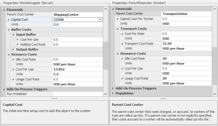
Figure 5.9: Financial properties on Server (left) and Worker.
The left side of Figure 5.9 illustrates an automated shrink wrapping machine (a Server). It requires a capital cost of 33,500 EUR, but the only cost of use is a fixed 13.852 EUR each time it is used. The shrink wrapper costs get rolled up to the Shipping Center cost center. The right side of Figure 5.9 illustrates a fork lift operator (a Worker) who gets paid 20 USD per hour whether busy or idle. But when the operator uses the fork lift to transport something it incurs an additional 31.50 USD per hour to account for the cost of the vehicle. The fork lift operator’s costs get rolled up to the Transportation cost center.
One final note is that multinational companies and projects often involve work being done across the world and hence in multiple currencies. Simio recognizes most common world currencies (I don’t think it yet handles goats or Bitcoins). The Financials category under the Advanced Options on the Run tab allows you to specify the exchange rate for the currencies you want to use as well as the default currency to be used in reports.
5.2 Model 5-1: PCB Assembly
Now that we have a better understanding of the Simio framework, we’ll return our focus to modeling and analysis. The models in this chapter relate to a simplified assembly operation for printed-circuit boards (PCBs). PCBs are principal components in virtually all electronics products. PCB assembly basically involves adding electronic components of various types to a special board designed to facilitate electronic signaling between the components. Figure 5.10 (Courtesy of the Center for Advanced Vehicle Electronics (CAVE) at Auburn University: cave.auburn.edu) shows an example printed-circuit board. PCB assembly generally involves several sequential-processing steps, inspection and rework operations, and packaging operations. Through this chapter, we’ll successively add these operations to our models, but for now, we’ll start with a straightforward enhancement to our single-server queueing models from Chapter 4.
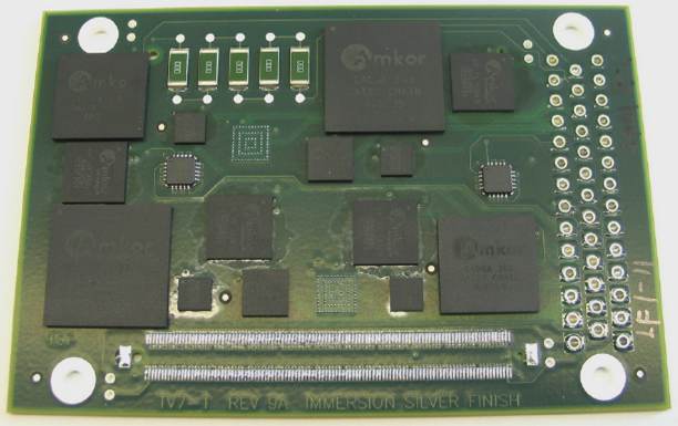
Figure 5.10: Example printed circuit board.
Model 5-1 focuses on a single operation where surface-mount components are placed on the board (the black rectangular shaped components on the board shown in Figure 5.10, for example) and the subsequent inspection operation. Boards arrive to the placement machine from an upstream process at the rate of 10 boards per hour (assume for the time being that the arrival process is Poisson, i.e., the interarrival times are exponentially distributed). The placement-machine processing times are triangularly distributed with parameters (3, 4, 5) minutes. After component placement, boards are inspected to make sure that all components were placed correctly. A human performs the inspection and the inspection times are uniformly distributed between 2 and 4 minutes. Historical records indicate that 92% of inspected boards are found to be “good” and the remaining 8% are found to be “bad.” Since the interarrival, component-placement, and inspection times are all random, we expect some queueing and we’d like to estimate the queue lengths and utilizations for the placement machine and the inspector. We’ll also estimate the time that boards spend in our small system and how much of this time is spent waiting, and we’ll count the number of good and bad boards.
We could (and some of you likely will) jump into the model building at this point, but it makes sense to spend a little effort developing some expectation about our system, since (as described in Section 4.2.5) we’ll need to verify our model before we can use it to estimate our performance metrics of interest. Recall that the basic verification process involves comparing your model results with your expectations. Figure 5.11 shows the basic queueing model of our initial PCB assembly system. Given the board arrival rate (\(\lambda = 10\)) and the respective service rates (\(\mu_{p} = 15\) and \(\mu_{i} = 20\)), all in units of boards per hour, we can compute the exact server utilizations at steady state (the utilizations are independent of the specific inter-arrival and processing time distributions). Since \(\rho_{p} = \lambda / \mu_{p} = 0.667 < 1\), we know that the arrival rate to the inspector is exactly 10 boards/hour (why?) and therefore, \(\rho_{i} = \lambda / \mu_{i} = 0.500\). Since both of the server utilizations are strictly less than 1, our system is stable (we can process entities at a faster rate than they arrive, so the number of entities in the system will be strictly finite, i.e., the system won’t “explode” with an ever-growing number of boards forever). If we assume that the placement and inspection times are exponentially distributed, we can also calculate the expected number of boards in our system, \(L = 3.000\) and the expected time that a board spends in the system, \(W = 0.3000\) hours (see Chapter 2 for details), both at steady-state, of course. While the times are not exponentially distributed, as we saw in Chapter 4 it’s easy to make them so initially in our simulation model in order to verify it.
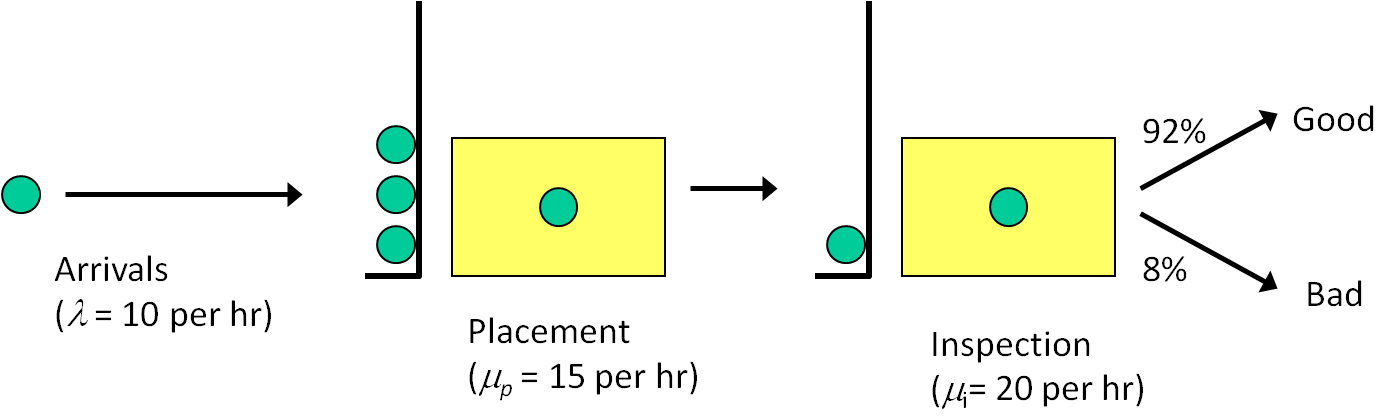
Figure 5.11: Example 5-1 queueing model.
Armed with our expectation, we can now build the Simio model. Compared to our models in Chapter 4, Model 5-1 includes two basic enhancements: sequential processes (inspection follows component placement); and branching (after inspection, some boards are classified as “good” and others are classified as “bad”). Both of these enhancements are commonly used and are quite easy in Simio. Figure 5.12 shows the completed Simio model, consisting of an entity object (PCB), a source object (Source1), two server objects (Placement and Inspection), and two sink objects (GoodParts and BadParts).
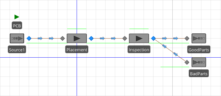
Figure 5.12: Model 5-1.
For our initial model, we used Connectors to connect the objects and specify the entity flow. Recall that a Connector transfers an entity from the output node of one object to the input node of another in zero simulated time. Our sequential processes are modeled by simply connecting the two server objects (boards leaving the Placement object are transferred to the Inspection object). Branching is modeled by having two connectors originating at the same output node (boards leaving inspection are transferred to either the GoodParts sink or the BadParts sink).
To tell Simio how to decide which branch to select for a given entity, we must specify the Routing Logic for the node, which Figure 5.13 illustrates for Model 5-1. Here, the output node for the Inspection object is selected and the Outbound Link Rule property in the Routing Logic group is set to By Link Weight. This tells Simio to choose one of the outbound links randomly using the connectors Selection Weight properties to determine the relative probabilities of selecting each link (note that Shortest Path is the default rule but only applies when the entity has a set destination. By Link Weight will be used if no entity destination is set even if the rule is set to Shortest Path).
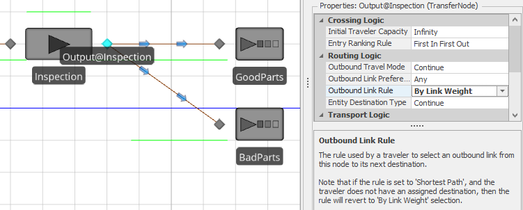
Figure 5.13: Output node Routing Logic.
Since our model specifications indicated that 92% of inspected boards are good, we set the Selection Weight property to 0.92 for the link to the GoodParts object (see Figure 5.14) and 0.08 for the link to the BadParts object. This link-weight mechanism allows us easily to model \(n\)-way random branching by simply assigning the relative link weight to each outgoing link. Note that we could have also used 92 and 8 or 9.2 and 0.8 or any other proportional values for the link weights — like a cake recipe 5 parts flour, 2 parts sugar, 1 part baking soda, etc. — Simio simply uses the specified link weights to determine the proportion of entities to route along each path. Simio includes several other methods for specifying basic routing logic — we’ll explore these in later models — but for now, we’ll just use the random selection.
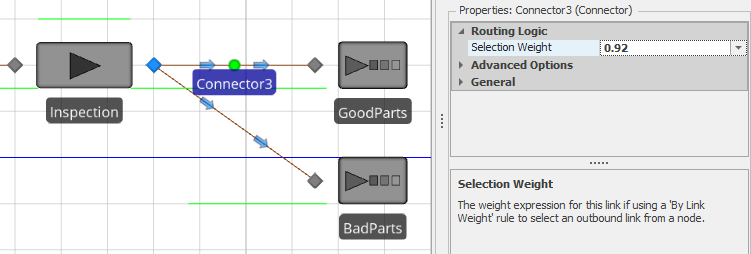
Figure 5.14: Selection weight for the link between the Inspection and GoodParts objects.
The final step to complete Model 5-1 is to specify the interarrival and service-time distributions using the Interarrival Time and Processing Time properties as we did in our previous models in Chapter 4. As a verification step, we initially set the processing times to be exponentially distributed so that we can compare to our queueing results. Table 5.2 gives the results from running 25 replications each with length 1200 hours and a 200 hour warm-up period. The results were all read from the Pivot Grid report as described in Section 4.2. These results are within the confidence intervals of our expectations, so we have strong evidence that our model behaves as expected (i.e., is verified). As such, we can change our processing time distributions to the specified values and have our completed model.
| Metric being estimated | Simulation |
|---|---|
| Placement Utilization (\(\rho_p\)) | \(0.666 \pm 0.004\) |
| Inspection Utilization (\(\rho_i\)) | \(0.498 \pm 0.003\) |
| Number in system (\(L\)) | \(2.992 \pm 0.060\) |
| Time in system (\(W\)) | \(0.280 \pm 0.005\) |
| Average number of “good” parts | \(9178.480 \pm 44.502\) |
| Average number of “bad” parts | \(803.280 \pm 11.401\) |
Table 5.3 gives the results based on the same run conditions as our verification run. Note that, as expected, the utilizations and proportions of good and bad parts did not significantly change but our simulation-generated estimates of the number of entities (\(L\)) and time in system (\(W\)) both went down (note that while the actual numbers did change, our estimates did not change in a probabilistic sense — remember that the averages and confidence-interval half widths are observations of random variables). Also, note that we should have expected these reductions as we reduced the variation in both of the processes when we switched from the exponential distribution to the triangular and uniform distributions (both of which, unlike the exponential distribution, are bounded on the right).
| Metric being estimated | Simulation |
|---|---|
| Placement Utilization (\(\rho_p\)) | \(0.668 \pm 0.002\) |
| Inspection Utilization (\(\rho_i\)) | \(0.501 \pm 0.002\) |
| Number in system (\(L\)) | \(1.849 \pm 0.020\) |
| Time in system (\(W\)) | \(0.185 \pm 0.002\) |
| Average number of “good” parts | \(9205.400 \pm 34.588\) |
| Average number of “bad” parts | \(806.320 \pm 12.357\) |
5.3 Model 5-2: Enhanced PCB Assembly
In this section, we’ll enhance our PCB assembly model to add features commonly found in real systems. The specific additional features include:
- Rework — Where the inspected boards were previously classified as either Good or Bad, we’ll now assume that 26% of inspected boards will require rework at a special rework station where an operator strips off the placed components. These rework boards all come out of what were previously deemed good boards, so that of the total coming out of inspection, 66% are now free-and-clear “good,” 8% are hopelessly “bad,” and 26% are rework. We’ll assume that the rework process times are triangularly distributed with parameters (2, 4, 6) minutes. After rework, boards are sent back to component placement to be re-processed. Reworked boards are treated exactly like newly arriving boards at the placement operation, and have the same good, bad, and rework probabilities out of all subsequent inspections (note that there’s no limit on the number of times a given board might be found in need of rework, and thus loop back through placement and inspection).
- Worker Schedules — The inspection and rework operations are both done by human operators, and we’ll explicitly consider the hours of the work day that the operators work and will include “meal breaks.” Inspection is done throughout the work day, but rework is done only during “second shift.” We continue to assume that placement is automated and requires no human operator.
- Machine Failures — The placement machine is an automated process and is subject to random failures where it must be repaired.
Since we have introduced the concept of worker schedules into our model, we must now explicitly define the work day. For Model 5-2, we assume that a work day is 24 hours and we will be running our model continuously for 125 of these days.
5.3.1 Adding a Rework Station
Figure 5.15 shows the completed model. To add the rework station, we simply added an new server object Rework, set the Processing Time and Name properties, and connected the input node of the server to the output node of the Inspection object, forming a 3-way branching process leaving inspection (be sure to update the link weights accordingly). Since reworked boards are sent back to the placement machine for processing, we connected the output node of the Rework object to the input node of the Placement object. This is our first example of a merging process. Here we have two separate “streams” of entities entering the Placement object — one from the Source1 object (newly arriving boards) and the other from the Rework object (boards that had previously been processed, failed inspection, and reworked). The Placement object (and its input node) will treat the arriving entities exactly the same, regardless of whether they arrived from the Source1 object or the Rework object. In a future model, we’ll demonstrate how to distinguish between arriving entities and treat them differently depending on their state.
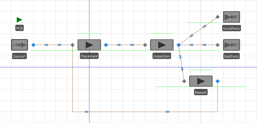
Figure 5.15: Model 5-2.
Given the structure of our system (and the model), it’s possible for PCBs to be reworked multiple times since we don’t distinguish between new and reworked boards at the placement or inspection processes. As such, we’d like to keep track of the number of times each board is processed by the placement machine and report statistics on this value (note that we could have just as easily chosen to track the number of times a board is reworked — the minimum would just be 0 rather than 1 in this case). This is an example of a user-defined statistic — a value in which we’re interested, but Simio doesn’t provide automatically. Adding this capability to our model involves the following steps:
- Define an entity state that will keep track of the number of times the entity has been processed in the placement machine;
- Add logic to increment that state value when an entity is finished being processed by the placement machine;
- Create a Tally Statistic that will report the summary statistics over the run; and
- Add logic to record the tally value when an entity departs the system (as either a good or bad part).
Note that this is similar to the TimeInSystem statistic that we modeled in Section 4.3. Both of these are examples of observational statistics (also called discrete-time processes), where each entity produces one observation — in the current case, the number of times the entity went through the placement process, and in Model 5-2, the time the entity spent in the system — and the Tally Statistic reports summary statistics like average and maximum over all observations (entities, in both cases). Note that the standard deviation is not not included in the summary statistics … see Section 3.3.1 for why doing so would often be biased and thus invalid, even though it easily could be done.
A state is defined within an object and stores a value that changes over the simulation run (Section 5.1.2.2). This is exactly what we need to track the number of times an entity goes through the placement process — every time the entity goes through (exits) the process, we increment the value stored in the state. In this case, we need to define the state with respect to the entity so we select the ModelEntity in the Navigation window, select the Definitions tab, select States from the Panel, and click on Integer icon from the ribbon (see Figure 5.16).
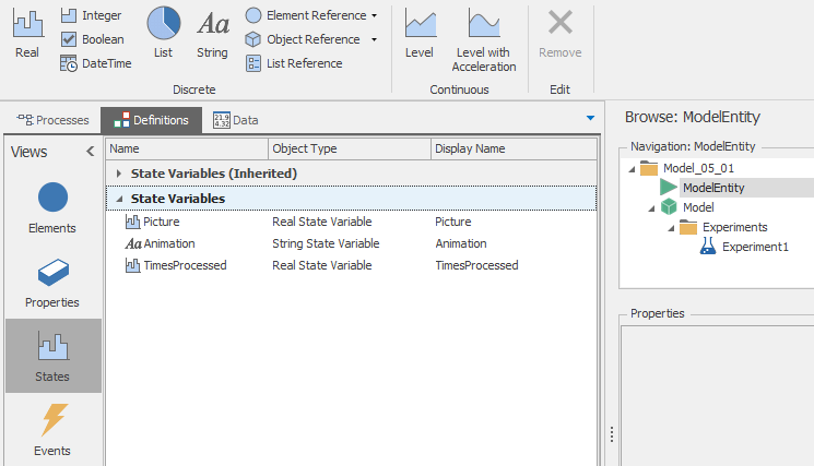
Figure 5.16: Creating the TimesProcessed entity state.
We named the state TimesProcessed for this model. Every entity object of type ModelEntity will now have a state named TimesProcessed and we can update the value of this state as the simulation runs. In our case, we need to increment the value (add 1 to the current value) at the end of the placement process. There are several ways that we could implement this logic in Simio. For this model, we’ll use the State Assignments property associated with Server objects. This property allows us to make one or more state assignments when an entity either enters or exits the server; see Figure 5.17.
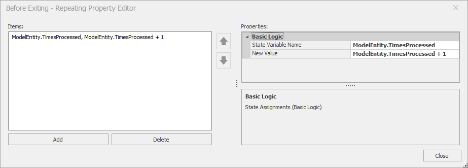
Figure 5.17: Setting the State Assignments property for the Placement object.
Here we’ve selected the Placement object, opened the Before Exiting repeat group property in the State Assignments section, and added our state assignment to increment the value of the TimesProcessed state. This tells Simio to make the specified set of state assignments (in our case, the single assignment) just before an entity leaves the object. So at any point in simulated time an entity’s TimesProcessed state indicates the number of times that entity has completed processing by the Placement object.
Next, we need to tell Simio that we’d like to track the value of the TimesProcessed state as an observational (tally) statistic just before entities leave the system. This is a two-step process:
- Define the tally statistic; and
- Record the value (stored in the TimesProcessed entity state) at the appropriate location in the model.
First we’ll define the tally statistic by selecting the Model in the Navigation window, clicking on the Definitions tab, and selecting the Elements pane, and clicking on the Tally Statistic icon on the Ribbon to add the statistic (see Figure 5.18). Note that we named the tally statistic NumTimesProcessed by setting the Name property. Finally, we’ll demonstrate two different methods for recording the tally values: Using an add-on process to record the value of the TimesProcessed state to the tally statistic; and using the Tally Statistics property of the input node of the Sink object (ordinarily, you’d use one method or the other in a model, but we wanted to demonstrate both methods for completeness).
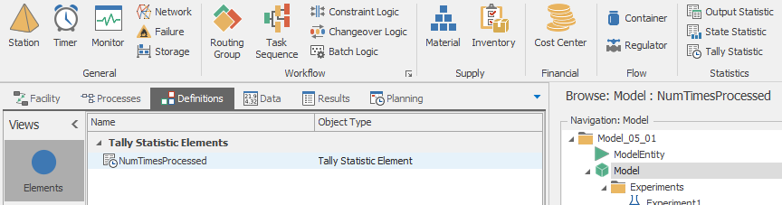
Figure 5.18: Creating the NumTimesProcessed tally statistic.
First, we’ll use the add-on process method for the entities that are routed to the GoodParts sink. The process will be executed when an entity enters the sink object. To create the add-on process, select the GoodParts Sink object and expand the Add-On Process Triggers group in the model properties panel. Four triggers are defined: Run Initialized, Run Ending, Entered, and Destroying Entity. Since we want to record each entity’s value in the tally, We chose the Entered trigger. You can enter any name that you like for the add-on process, but there is a nice Simio shortcut for defining add-on processes. Simply double-click on the trigger property name (Entered, in this case) and Simio will define an appropriate name and open the processes panel with the newly created process selected. The add-on process in this case is quite simple — just the single step of recording the tally value to the appropriate tally statistic. This is done using the Tally step (as shown in Figure 5.19).
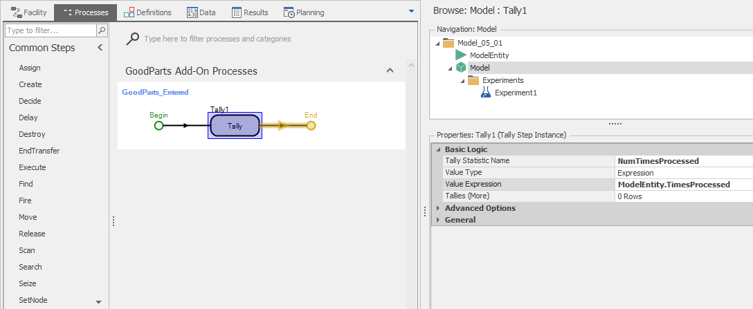
Figure 5.19: Add-on process for the GoodParts sink.
To add the step, simply select and drag the Tally step from the Common Steps panel onto the process and place it between the Begin and End nodes in the process. The important properties for the Tally step are the TallyStatistic Name, where we specify the previously defined Tally Statistic (NumTimesProcessed) and the Value, where we specify the value that should be recorded (the TimesProcessed entity state in this case). We also set the Value Type property to Expression to indicate that we’ll be using an expression to be evaluated and recorded.
The second method uses the Tally Statistics property for the Basic Node from the Standard Object Library and we’ll use this method with the Bad Parts sink. Figure 5.20) illustrates this method. First select the input node of the BadParts sink and expand the Tally Statistics property group (shown at the top of the figure). Next, open the repeat group editor by clicking on the ellipsis next to the On Entering property and add the tally as show in bottom part of the figure. Note that we use the same tally statistic for both part types since we wanted to track the number of times processed for all parts. Had we wanted to track the statistics separately by part type (Good and Bad), we would have simply used two different Tally Statistics. Now when we run the model, we’ll see our Tally statistic reported in the standard Simio Pivot Grid and Reports and the values will be available in case we wish to use them in our process logic.
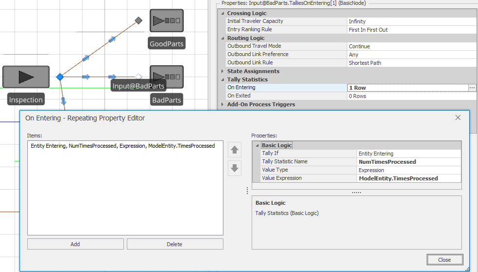
Figure 5.20: Using the Tally Statistics property for the input node of the BadParts sink object.
The process that we just described for creating a user-defined observational statistic is a specific example of a general process that we will frequently use. The general process for creating user-defined observational (tally) statistics is as follows:
- Identify the expression to be observed. Often, this involves defining a new model or entity state where we can compute and store the expression to be observed (as it did with the previous example);
- Add the logic to set the value of the expression for each observation, if it is not already part of the model;
- Create the Tally Statistic; and
- Tell Simio where to record the expression value using the Tally step in an add-on process or a Tally Statistic property for a node object instance at an appropriate location in the model.
We will follow this same general process wherever we incorporate user-defined observational statistics.
5.3.2 Using Expressions with Link Weights
Before continuing with Model 5-2, we would like to demonstrate using expressions for connector link weights. This is a very powerful, but often overlooked feature that can simplify the logic associated with link selection. Above, we specified fixed probabilities for the three possible inspection outcomes (good: 66%, rework: 26%, bad: 8%) and set the link weights accordingly. Suppose that we would like to limit the number of times that a board can be processed. For example, suppose that we had the following rules:
- Boards can be processed a maximum of 2 times. Any board processed a third time should be rejected;
- 95% of inspected board are good;
- 5% of inspected boards are bad.
and we would like implement this logic in our model. In this case, the link selection is not totally probabilistic. Instead there is a condition that determines whether the board should be rejected (it’s been processed 3 times) and, if that condition is not met, probabilities are used to determine between the remaining two alternative. Figure 5.21 shows a simple way to implement this logic using expressions for link weights. Note that the parenthetical components if the link weights will evaluate to either 0 or 1, so the probabilities are applied only if the board has been processed fewer than 3 times. Otherwise, the board will be rejected. This simple example illustrates the power of using expressions with the link-weight selection rule. New users will often unnecessarily resort to using more complex add-on processes in order to implement this type of logic. We encourage to you study this example carefully as these types of expressions can greatly simplify model development. Of course, if we were really implementing this system, we would like to reject the board before it is processed the third time – i.e., immediately after it fails inspection for the second time, but before it is reworked. We leave this as an exercise for the reader (see Problem 7 at the end if the chapter).
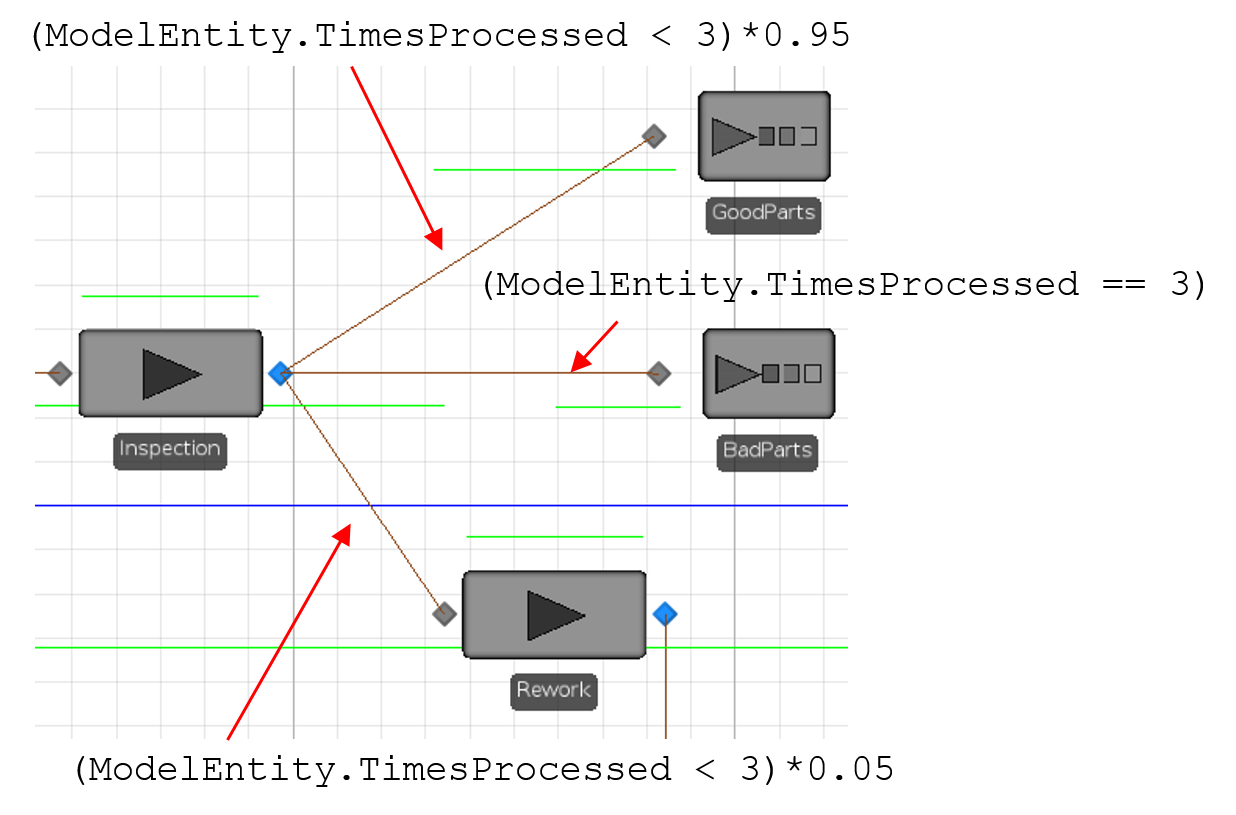
Figure 5.21: Example of using expressions with link weights.
5.3.3 Resource Schedules
The rework and inspection operations of our PCB assembly system are both performed by human operators (the placement process is still automated). Human operators generally work in shifts and take breaks during the work day. Before describing how to implement worker schedules in Simio, we must first describe how Simio tracks the time of day in simulated time. Simio runs are based on a 24-hour clock with each “day” starting at 12:00 a.m. (midnight) by default. In our previous models, we’ve focused on the replication run length and warm-up period length, but have not discussed how runs are divided into 24-hour days.
In our PCB example, we’ll assume that the facility operates three 8-hour work shifts per day and that each shift includes a 1-hour meal break (so a worker’s day is actually 9 hours including the meal break). The shifts are as follows.
- First shift: 8:00 a.m. – 12:00 p.m., 12:00 p.m. – 1:00 p.m. (meal break), 1:00 p.m. – 5:00 p.m.
- Second shift: 4:00 p.m. – 8:00 p.m., 8:00 p.m. – 9:00 p.m. (meal break), 9:00 p.m. – 1:00 a.m.
- Third shift: 12:00 a.m. – 4:00 a.m., 4:00 a.m. – 5:00 a.m. (meal break), 5:00 a.m. – 9:00 a.m.
We’ll also assume that, for multi-shift processes (inspection, in our case), a worker’s first hour is spent doing paperwork and setting up for the shift, so that there’s only one worker actually performing the inspection task during those periods when worker shifts overlap.
Given the work schedule that we described, the inspection operation operates 24-hours per day with three 1-hour meal breaks (12:00 noon – 1:00 p.m., 8:00 p.m. – 9:00 p.m., and 4:00 a.m. – 5:00 a.m.). This schedule would correspond to having three inspection operators, each of whom works 8 hours per day. Since Simio is based on a 24-hour clock that starts at 12:00 a.m., this translates to the inspection resource capacity schedule shown in Table 5.4.
| Time period | Resource Capacity |
|---|---|
| 12:00 a.m. – 4:00 a.m. | 1 |
| 4:00 a.m. – 5:00 a.m. | 0 |
| 5:00 a.m. – 12:00 p.m. | 1 |
| 12:00 p.m. – 1:00 p.m. | 0 |
| 1:00 p.m. – 8:00 p.m. | 1 |
| 8:00 p.m. – 9:00 p.m. | 0 |
| 9:00 p.m. – 12:00 a.m. | 1 |
With this work schedule, we’d expect boards to queue in front of the inspection station during each of the three “meal periods” when there is no inspector working. Once we complete the model, we should be able to see this queueing behavior in the animation. There are multiple ways to implement this type of resource capacity schedule in Simio — for Model 5-2, we’ll use Simio’s built-in Schedules table. To use this table, we first define the schedule and then tell the Inspection object to use the schedule to determine the object’s resource capacity.
To create our work schedule, select the Model in the Navigation pane, select the Data tab, and the Schedules icon in the Data panel. You’ll see two tabs — under the Work Schedules tab you’ll see that a sample schedule named StandardWeek has already been created for you, and under the Day Patterns tab you’ll see that a sample StandardDay has been created for you.
We’ll start under the Day Patterns tab to define the daily work cycle by telling Simio the capacity values over the day. We can choose either to revise the sample pattern, or to replace it. Select StandardDay and then click on Remove to delete the existing pattern, then click on Day Pattern in the Create category of the ribbon to create a new one. Give the new pattern a Name of DayPattern1 and click the + to the left of it to expand the Work Periods definition. In the first work period row, type or use the arrows to enter 12:00:00 AM for Start Time then type 4 for the Duration. You’ll see that End Time is automatically calculated and that the Value (capacity of the resource) defaults to 1. Continue this process to add the three additional active work periods as indicated in Table 5.4. Your completed day pattern should look like that in Figure 5.22.
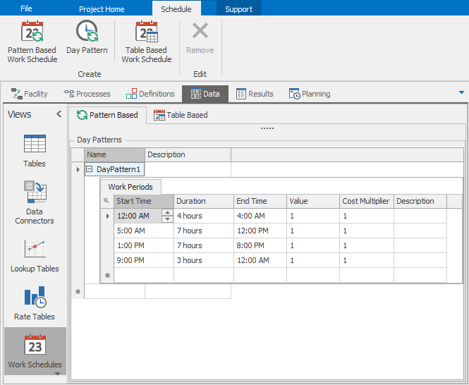
Figure 5.22: Definition of inspection day pattern.
Now let’s move back to the Work Schedules tab. Again, we could delete the sample schedule and create a new schedule, but this time we’ll just change it to meet our needs. Change the Work Schedule Name to InspectionSchedule and change the Description to Daily schedule for inspectors. For our model, the work pattern is the same every day so we’ll set the Days property value to 1 to indicate that the same pattern will repeat every (one) day. Finally, since we deleted the StandardDay pattern that was originally referenced here, the Day 1 column indicates an error. To clear the error, just select the new DayPattern1 from the pull-down list. Your completed work schedule should look like that in Figure 5.23.
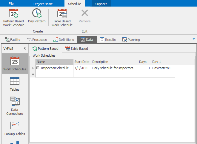
Figure 5.23: Inspection schedule.
Now that we have the schedule defined, we tell the Inspection object to use the schedule to specify the resource capacity. We can do this by selecting the Inspection object and setting the Capacity Type property to WorkSchedule and setting the Work Schedule property to InspectionSchedule (see Figure 5.24).
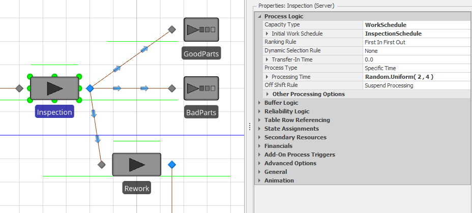
Figure 5.24: Specifying a WorkSchedule for the Inspection object.
Next, we need to specify the capacity schedule similarly for the rework operator. As specified above, the rework operation works only during the second shift, which will be 4:00 p.m. – 8:00 p.m., 8:00 p.m. – 9:00 p.m. (meal break), and 9:00 p.m. – 1:00 a.m. So, as before, we created a new day pattern DayPattern2 and referenced that day pattern in a new work schedule ReworkSchedule and then told the Rework object to use the schedule (see Figure 5.25).
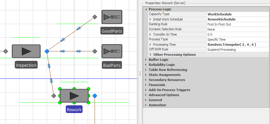
Figure 5.25: Specifying a WorkSchedule for the Rework object.
Schedules will be discussed in more detail in Section 7.2.
Before incorporating the placement-machine failures into our model, it’s instructive to consider how incorporating resource capacity schedules affects our server-utilization statistics. In our previous models, we defined the utilization as the proportion of the run in which the server was busy (or the percentage resulting from multiplying the proportion by 100). This worked because the capacity of the server resources did not change throughout the run. Now that we have servers where the resource capacity changes over the model run, the utilization calculation is a bit more difficult — in fact, the interpretation of utilization itself is no longer straightforward. In particular, it’s not clear how to account for the “off-shift” time for the server resources. As an example, assume that the rework operator is busy \(6.28\) hours for a particular day. One method of computing utilization involves dividing the busy time by the day length (24 hours), yielding a utilization of \(26.17\%\). However, if you were the rework operator, you’d likely say “Wait a minute, I was way busier than that!” The problem (from the operator’s perspective) is that the utilization calculation doesn’t take into consideration that the rework operator is only available 8 hours of every 24-hour day (i.e., only during second shift). As a second calculation, we could divide the busy time by the 8 hours that the operator is actually available, yielding a utilization of \(78.50\%\) — a value with which the rework operator would likely agree. Note that neither of these interpretations is technically “incorrect,” they are simply two different interpretations of the concept of resource utilization, and Simio provides both as part of its default output.
Figure 5.26 shows a portion of the standard Pivot Grid report from a run of 25 replications of Model 5-2 (without the placement-machine failures) of run length 125 days with a 25-day warm-up period. The portion of the Pivot Grid shows the Server Resource statistics for the Inspection object. The values in which we’re particularly interested for our utilization discussion are extracted to Table 5.5.
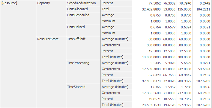
Figure 5.26: Resource section of the Pivot Grid for the Inspection object.
| Category | Statistic | Value |
|---|---|---|
| Capacity | ScheduledUtilization (Percent) | 77.3062 |
| UnitsScheduled (Average) | 0.8750 | |
| UnitsUtilized (Average) | 0.6764 | |
| Resource State | Offshift Time (Percent) | 12.5000 |
| Processing Time (Percent) | 67.6429 | |
| Starved Time (Percent) | 19.8571 |
The statistics are defined as follows.
- ScheduledUtilization (Percent) — The percent utilization of the object’s scheduled capacity during the run, calculated by returning the value of the expression \(100 * (Capacity.Utilized.Average/Capacity.Average)\).
- UnitsScheduled (Average) — The average scheduled capacity of this object during the run.
- UnitsUtilized (Average) — The average number of capacity units of this object that have been utilized during the run.
- Offshift Time (Percent) — The percentage of the run during which the resource is in the Offshift state.
- Processing Time (Percent) — The percentage of the run during which the resource is in the Processing state.
- Starved Time (Percent) — The percentage of the run during which the resource is in the Starved state. Note that starved in this context means that the resource is available to work, but there are no entities available to process.
In our simple example above involving the rework operator, the \(26.17\%\) measure is equivalent to the \(UnitsUtilized * 100\) and the \(78.50\%\) is equivalent to the ScheduledUtilization. Similarly, the values in Table 5.5 tell us that the inspection operators are busy roughly 77.3% of the time that they are working, and that there is an inspection operator busy roughly 67.7% of the entire day. The UnitsScheduled value of 0.8750 is based on the fact that the three 1-hour meal breaks mean that inspection operators are scheduled to be available 21 out of the 24 hours each day (or 0.8750 of the day).
Note that there will not always be the same relationship between the Capacity values and the Resource State values. In particular, the following relationships hold because the resource capacity values in the schedule were either 0 or 1.
\[Average~UnitsScheduled = \frac{Processing~Time~\% + Starved~Time~\%}{100}\]
\[Average~UnitsUtilized = \frac{Processing~Time~\%}{100}\]
If the resource capacities are greater than 1 during a schedule (e.g., if some shifts had 2 or 3 inspectors working), the Resource State values are independent of the number of units of a resource that are busy, whereas the Capacity values take the specific numbers of units of resource capacity into consideration. For example, if we halve the inspection processing rate (set the Processing Time property to Random.Uniform(4, 8)) and change the schedule so that there are 2 inspectors rather than 1 during the work cycles, we get the results shown in Table 5.6.
| Category | Statistic | Value |
|---|---|---|
| Capacity | ScheduledUtilization (Percent) | 77.4024 |
| UnitsScheduled (Average) | 1.7500 | |
| UnitsUtilized (Average) | 1.3545 | |
| Resource State | Offshift Time (Percent) | 12.5000 |
| Processing Time (Percent) | 82.5084 | |
| Starved Time (Percent) | 4.9916 |
In this model, the ScheduledUtilization and Offshift Time percentage did not change (as we’d expect — make sure you understand why this is true!), but the other values did. The ProcessingTime percentage went up because it measures the percentage of time that either or both of the units of capacity are busy. Similarly, the Starved Time percentage went down because now both units of capacity have to be starved in order for the inspection resource to be in the starved state.
5.3.4 Machine Failures
The final enhancement for Model 5-2 is to incorporate random machine failures for the placement machine (note that we also gave a machine-failure example in Section 5.1.4). As with most complex mechanical devices, the placement machine is subject to failures where it must be repaired before in can continue processing boards. Simio’s Server object from the Standard Library supports three different types of failures:
- Calendar Time Based — the uptime is based on calendar time and you specify the uptime between failures;
- Event Count Based — the uptime is based on the number of times an event occurs and you specify the number of events; and
- Processing Count Based — the uptime is based on the number of times the server processes an entity and you specify the number of times that the server processes between failures.
For our placement-machine failures, we’ll use the Calendar Time Based failures. Historical records show that our placement machine fails after about 6 hours of uptime and that the time required to repair the machine after it fails is approximately 30 minutes. As both the uptime and repair durations are highly variable, we’ll assume that both are exponentially distributed. To incorporate this failure model into Model 5-2, we need to set the Failure Type property to Calendar Time Based, the Uptime Between Failures property to Random.Exponential(6) Hours, and the Time to Repair property to Random.Exponential(30) Minutes (see Figure 5.27).
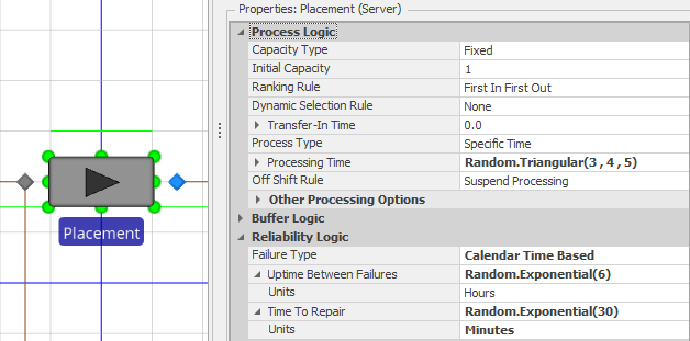
Figure 5.27: Defining the failures for the placement object.
Now when we run the model (using the same run parameters as in the previous section), we can see that the ResourceState category for the Placement object now includes a section for Failed Time (see Figure 5.28) and that our estimate of the percentage of time that the machine spends in the failed state is approximately \(7.54\%\).
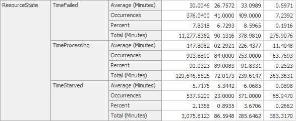
Figure 5.28: Placement resource state results after adding failures.
Calendar Time Based failures are most commonly used to model random mechanical failures where the time between failures is a function of time. Processing Count Based failures are most commonly used to model failures where the time between failures is a function of the number of times the process is used. Raw-material replenishment is an example of a situation that would call for this type of failure process. In this situation the machine has an inventory of raw materials that is exhausted by processing parts. When the raw-material inventory is empty, the machine can’t continue processing until the raw-material inventory is replenished. As such, the time between failures will be a function of the number of parts processed (or, more specifically, the Processing Count). Event Count Based failures are based on the number of occurrences of an event, which can be a standard Simio-defined event or a user-defined event.
5.3.5 Verification of Model 5-2
Before using our model to analyze our system, we need to have some confidence that our model is “correct.” In the current context, this involves verifying that our model behaves as expected (i.e., that we’ve correctly translated the specifications into our working Simio model). When we verified Model 5-1 and the models in Chapter 4, our basic strategy was to develop some expectations to which we could compare the model output. However, in those models, the queueing analysis that we used to develop our expectation was very straightforward. With Model 5-2, we’re beginning to add model components that are difficult to incorporate into standard queueing models even though Model 5-2 is still a very simple model. Of course we expected this — if we could completely analyze systems using queueing (or other analytical methods), there would be no need for simulation! The two components that complicate our queueing analysis of Model 5-2 are:
- Re-entrant flow — Since the boards that leave the rework station are sent back for re-processing, the arrival rate to the Placement station will be greater than the external arrival rate of 10 boards/hour; and
- Resources changing capacity during the run — With the incorporation of resource-capacity schedules and machine failures, the capacities of the Placement, Inspection, and Rework resources will vary over time.
We’ll consider these issues one at a time. Since the arrival rate to the Placement station will be greater than the 10 boards/hour we had in Model 5-1, we expect the Placement resource utilization also to be higher. To estimate the new utilization, we need to determine (or estimate) the new arrival rate. Figure 5.29 illustrates the re-entrant flow.
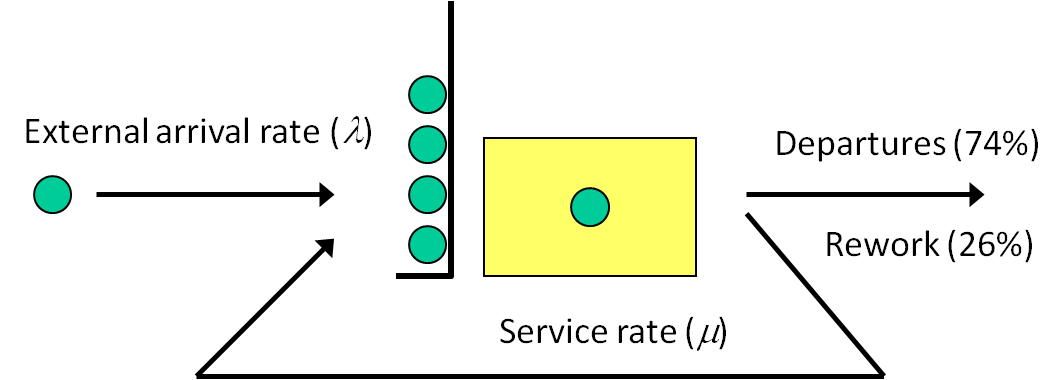
Figure 5.29: Re-entrant flow.
If we let \(\lambda'\) be the effective arrival rate (i.e., the arrival rate that the process actually sees), then:
\[\begin{eqnarray*} \lambda' & = \lambda + 0.26\times\lambda' \end{eqnarray*}\]
Solving for \(\lambda'\), after a few steps of algebra, we get:
\[\begin{eqnarray*} \lambda' & = \lambda /(1 - 0.26) \\ & = 1.3514\times\lambda \end{eqnarray*}\]
Ignoring the machine failures for now, we’d expect the utilization of the placement machine to be \(13.514 / 15 = 0.9019\). Since the utilization is strictly less than 1, the departure rate will equal the arrival rate and the expected utilization for the inspection station will be \(13.514 / 20 = 0.6757\) (ignoring the resource-capacity schedule). Similarly, since the inspection utilization is also strictly less than 1, the expected utilization for the rework station will be \((13.514 \times 0.26) / 15 = 0.2342\) (again, ignoring the resource-capacity schedule). If you run Model 5-2 ignoring the resource-capacity schedules and machine failures, you’ll see that the model matches our expectation.
The resource-capacity schedules and the machine failures will have the effect of reducing the available capacities of the resources. For the resource-capacity schedules, it’s instructive to consider the daily arrival and service rates for the inspection and rework operations. Since the inspection operators work a combined 21 hours/day (due to the three one-hour meal breaks), the daily processing rate is \(21 \times 20 = 420\) and the expected utilization is \((24 \times 13.514) / 420 = 0.7722\). Similarly, since the inspection operator works only during second shift, the daily processing rate is \(8 \times 15 = 120\) and the expected utilization is \((24 \times 13.514 \times 0.26) / 120 = 0.7027\).
We’ll take a slightly different approach for the machine failures. Recall that the expected uptime for the placement machine is 6 hours and the expected time to repair it is 30 minutes. As such, the machine is failed for approximately 30 minutes out of every 390 minutes, or \(7.692\%\) of the time. Since the expected percentage of time that the placement machine is idle (\((1 - 0.9010) \times 100 = 9.91\%)\) is greater than the expected percentage of failed time, we’d expect the system to remain stable.
Table 5.7 gives the pertinent results based on 50 replications of 600-day runs with 100-day warmup. As these values appear to match our expectation, we have strong evidence that our model is correct (verified) and we can now use the model to analyze the system.
| Metric being estimated | Simulation |
|---|---|
| Placement Utilization (\(\rho_p\)) | \(0.9006 \pm 0.0825\) |
| Inspection Utilization (\(\rho_i\)) | \(0.7719 \pm 0.0716\) |
| Rework Utilization (\(\rho_4\)) | \(0.7025 \pm 0.1198\) |
| Percent failed time (placement) | \(7.6926 \pm 0.0591\) |
5.4 Model 5-3: PCB Model With Process Selection
The final enhancement that we’ll add to our PCB model involves adding a second component-placement process immediately after our current placement process. The second placement process will add fine-pitch components to the PCB. Because of the placement-location accuracy required by these components, the placement process takes significantly longer than does the regular component-placement process. As such, we’ll use three placement machines in parallel so that the fine-pitch placement process will be able to keep up with the regular placement, inspection, and rework processes. Figure 5.30 shows the completed model. Note that this is a common configuration for serial production systems that include processes with different speeds.
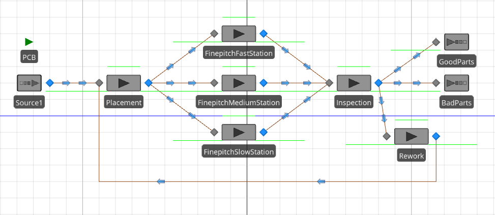
Figure 5.30: Model 5-3.
Just to make the model interesting, we’ll also assume that the three fine-pitch placement machines are not identical. More specifically, we’ll assume that we have a fast machine, a medium machine, and a slow machine where the processing times are random and are distributed as follows:
- Fast — Triangular(8, 9, 10);
- Medium — Triangular(10, 12, 14); and
- Slow — Triangular(12, 14, 16).
Finally, we’ll also assume that the fast machine is subject to random failures with the up times’ being exponentially distributed with mean 3 hours and repair times’ being exponentially distributed with mean 30 minutes. Note that for this model, we assume that the medium and slow machines do not fail.
As shown in Figure 5.30, we removed the Connection object between the Placement object and the Inspection object and added three new server objects representing the three fine-pitch placement machines (FinepitchFastStation, FinepitchMediumStation, and FinepitchSlowStation). We set the Capacity Type property to Fixed and the Initial Capacity property to 1 for each station and we set the Processing Time properties to the specified processing-time distributions given above. For the FinepitchFastStation object, we also added the failures (see Figure 5.31).
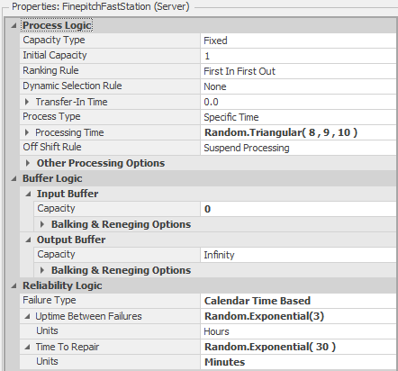
Figure 5.31: FinepitchFastStation object properties.
We next connected the output node of the Placement object to the input nodes of the three new server objects using Connector objects (branching) and similarly connected the output nodes of the new server objects to the input node of the Inspection object (merging).
The model now has five server object instances and it’s an opportune time to demonstrate the use of the properties spreadsheet view. This view presents the common properties of all instances of a given object in familiar spreadsheet format. Figure 5.32 shows Model 5-3 with the properties spreadsheet view open. You can open the properties spreadsheet view by right-clicking on an object instance and choosing the Open properties spreadsheet view for all objects of this type ... option from the context menu. You can also open the view using the Properties button from the Windows section of the Project Home ribbon. The properties spreadsheet view includes the same standard sorting and filtering options that other spreadsheet views include and it can be quite useful for models with multiple instances of the same objects.
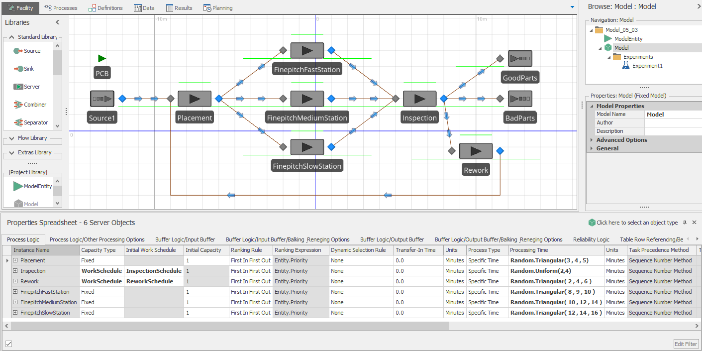
Figure 5.32: Spreadsheet properties view for Model 5-3.
In our first example of branching in Section 5.2, we used link weights to select randomly between the alternative entity destinations. We could easily use this same logic to select the fine-pitch machine, but this is likely not what we want. Rather than selecting the machine randomly, we’d like to select the “first available” machine. We’ll use a Simio node list to implement this logic. In order to use the node list, we must first define the list and then tell the Placement object’s output node to use the list to determine the destination for the PCB objects. To define the list, select the Model in the Navigation pane, select the Definitions tab, and the Lists icon from the Definitions panel. Note that Simio supports String, Object, Node, and Transporter lists. Click on the Node icon in the Ribbon to create a new node list and then add the input nodes for the three fine-pitch objects (Input@FinepitchFastStation, Input@FinepitchMediumStation, and Input@FinepitchSlowStation) to the node list in the bottom pane of the main window (see Figure 5.33). Note that each of the Node list items in the bottom pane is selected from a pull-down list that includes all of the nodes in the model.
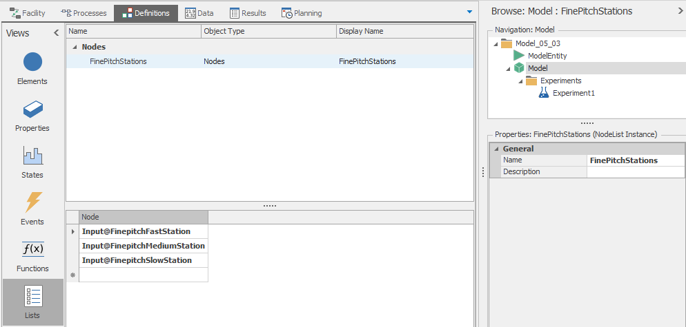
Figure 5.33: FinePitchStations node list.
Now that we have the list defined, we need to tell Simio how to select one of the list elements. In the real system, we’d like to send the PCB to the machine that will be available first. Since the processing times are random and the machines are subject to random failures, we won’t know for sure which one will be available first, so we’ll use a surrogate measure — we’ll select the machine with the fewest boards already waiting for or en route to the machine. To implement this logic, select the output node for the Placement object and set the parameters to the values shown in Figure 5.34.
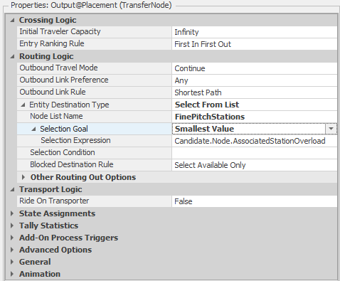
Figure 5.34: Properties for the output node of the Placement object.
The Entity Destination Type and Node List Name properties tell Simio to use the FinePitchStations list (Figure 5.33) and the Selection Goal property indicates that the smallest value of the Selection Expression. So, when an entity arrives at the node, Simio will evaluate the expression for each of the candidate nodes in the list, and will route the entity to the node with a minimum value of that expression.
The expression value, Candidate.Node.AssociatedStationOverload requires some explanation. The Candidate.Node keyword indicates that we want to consider each candidate node from the list. The AssociatedStationOverload function returns the Overload for each of the stations associated with the nodes (the fine-pitch machine objects, in our case). The AssociatedStationOverload property is defined in the Simio Reference Guide as:
- “For an external input node, returns the current difference between the load and capacity values (a positive difference indicating an `overload’) for the station locations inside the node’s associated object that may be entered using the node.
- The associated station `load’ is defined as the sum of entities currently en route to the node intending to enter the stations, plus the current number of entities arrived to the node but still waiting to enter the stations, plus the current number of entities occupying the stations. This function returns the difference between that load and the current station capacity (Overload = Load - Capacity).”
So when an entity reaches the output node of the Placement object, Simio will select the input node for the fine-pitch machine that has minimum overload (a measure of the workload waiting for the machine, in our context) and then route the entity to that node. If there are multiple nodes with the same overload value (e.g, when the first board arrives, all three machines are empty and idle), Simio will select the node based on the list order (i.e., the first node with the minimum value). Important Note: Functions like AssociatedStationOverload and AssociatedStationLoad don’t work well when Input Buffer Capacity is Infinity. You might recall from basic math that Infinity plus anything equals Infinity. So when infinite capacity queues are involved, a tie will result. For our problem, we put the fast machine first so that it would have priority in the case of ties and we set the buffer capacities to 0. By setting the capacities to 0, the decision of which destination to pick will be delayed as long as possible. You should also experiment with other finite buffer capacities like 1, 2, 3 to see the impact on the model behavior. In addition to AssociatedStationOverload, the AssociatedStation keyword can be used in combination with many values associated with the station. Common uses include (you can see and select from the alternatives by opening the value in the expression builder and using the down arrow to open the display):
- AssociatedStation.Capacity — For an external input node, returns the current capacity of the station;
- AssociatedStation.Capacity.Remaining — For an external input node, returns the current available (unused) capacity of the station;
- AssociatedStation.Contents — For an external input node, returns the number of entities currently waiting in the station;
Now that the logic for the fine-pitch placement process has been incorporated into our model, we’ll add one more set of user-defined statistics so that we can track the proportion of times that the fast, medium, and slow machines are selected, respectively. We do this for two reasons: first, for model verification — we expect approximately 38%, 33%, and 29% of the processing to be done by the fast, medium, and slow machines, respectively (see Problem 8 at the end of the chapter); and second, to demonstrate how to set up another user-defined statistic. The steps for creating the user-defined statistics are:
- Define a model state to record the number of times each machine is used to process a board;
- Increment the corresponding model state when one of the fast-pitch machines completes processing; and
- Tell Simio to report an Output Statistic for each proportion.
For the first step, select the Model in the Navigation window, select the Definitions tab, and the States icon from the Definitions panel. Then add the three Discrete States (NumFast, NumMedium, and NumSlow — see Figure 5.35).
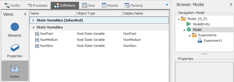
Figure 5.35: Defining the model states to track the fast-pitch machine process counts.
Note that when we defined the user statistic to track the numbers of times boards are processed by the placement machine (Section 5.3.1), we used an entity state rather than a model state. This was because we were tracking an entity characteristic in that case, whereas we’re tracking a model characteristic in this case. This is a very important distinction when you’re creating user-defined statistics. For the second step, we’ll use the same method that we used in Section 5.3.1 — we’ll use the State Assignments property associated with the Server objects and will increment the NumFast, NumMedium, and NumSlow states in the respective BeforeExiting repeat group. Finally, select the Elements icon from the model Definitions Panel and add the three Output Statistics to compute the proportion of processing steps completed by each machine. Recall that an Output Statistic reports the value of an expression at the end of a replication. The expression for the proportion of times the fast machine is used is:
\[NumFast/(NumFast+NumMedium+NumSlow)\]
This will tell Simio to compute the proportion at the end of the replication and to keep track of and report the statistics across replications. The output statistics for the medium and slow machine are similarly defined except we replace the NumFast in the numerator with NumMedium and NumSlow, respectively. Note that if the model terminates before any boards are processed, the denominator will evaluate to \(0\) and Simio will report a divide-by-zero error. To prevent this, we could use the Math.Max() function to ensure that the denominator is never \(0\) (e.g., Math.Max(1, NumFast + NumMedium + NumSlow)). This is generally good practice unless you want Simio to throw the error if the condition exists for some reason.
We could also have tracked the proportion statistics by defining the output statistics using the Simio-provided processing counts. In particular, the Simio property
\[FinepitchFastStation.Processing.NumberExited\] gives the number of entities that exit the FinepitchFastStation object. As such, the same proportion we specified above could be specified using the expression
\[\begin{eqnarray*} FinepitchFastStation.Processing.NumberExited / \\ (FinepitchFastStation.Processing.NumberExited+ \\ FinepitchMediumStation.Processing.NumberExited+ \\ FinepitchSlowStation.Processing.NumberExited) \end{eqnarray*}\]
Comparing these two methods, the benefit of using your own states is that you know exactly how the values are tracked and you can customize them as you see fit, but using the Simio-provided states is somewhat easier (since you don’t have to define or increment the states). It’s important to know how to use both methods — defining your own states and using Simio’s built-in states. Note that the possibility for division-by-zero error exists here also, so we should consider using the Math.Max() function as discussed above.
5.5 Model 5-4: Comparing Multiple Alternative Scenarios
One of the primary uses of simulation is to evaluate alternative system designs. For example, suppose that we are considering purchasing an additional fine-pitch placement machine for our PCB assembly system and we would like to know whether to purchase an additional fast machine, medium machine, or slow machine (presumably, these would cost different amounts). In this section, we’ll create Model 5-4 by modifying Model 5-3 so that we can compare the predicted performance of the system under each of these alternative designs. While we could easily modify the model to add capacity to one of the fine-pitch stations, run the model, save the results, repeat two additional times (changing the capacity of a different fine-pitch station each time), and manually compare the alternatives using the saved results, we’ll take a different approach that demonstrates the power of Simio’s experiment facilities. The first step is to define Referenced Properties (see Section 5.1.2.4) for the Initial Capacity properties for the three fine-pitch server objects so that we can easily manipulate the respective server capacities in our experiment.
Figure 5.36 shows the properties for the FinepitchFastStation server with the Initial Capacity property set to the referenced property InitialCapacityFast (note the green arrow indicating that the property value is a referenced property). To define a referenced property and set the Initial Capacity server property to this referenced property in a single step, simply right-click on the Initial Capacity property label in the Properties window (make sure you’re on the label and not the property), select Set Referenced Property from the pop-up menu, and select Create New Referenced Property from the bottom of the menu. This will bring up a dialog box where you enter the Reference Property name (we used InitialCapacityFast). Next, follow the same procedure to define the referenced properties for the medium and slow fine-pitch servers.
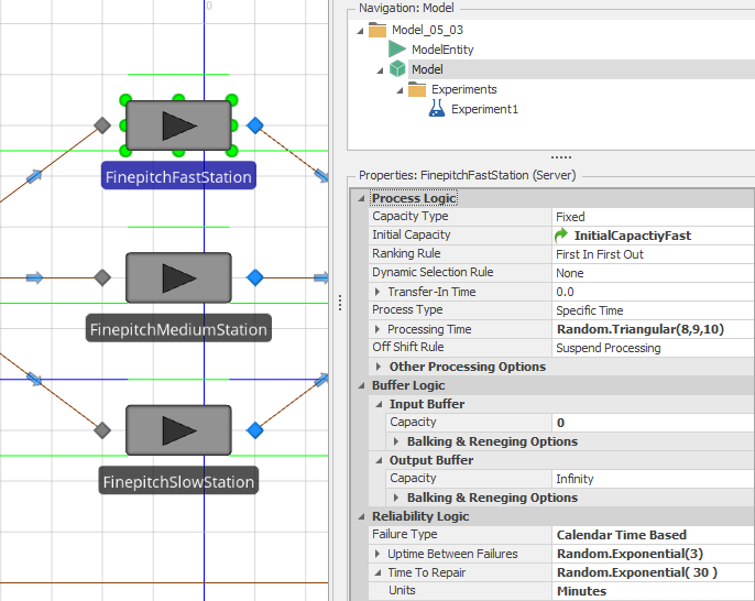
Figure 5.36: Setting the referenced property for the fast fine-pitch station.
After defining the three referenced properties, select the Model from the Navigation window, select the Definitions tab and the Properties panel to display the newly defined Reference Properties (see Figure 5.37).
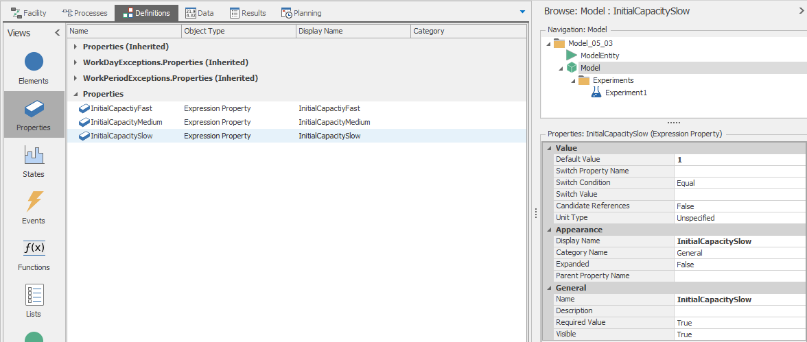
Figure 5.37: Referenced properties for Model 5-4.
This is where we set the Default Value property (set to 1 in Model 5-4). At this point, we have defined the new referenced properties and told Simio to use these properties to define the Initial Capacity properties for the three fine-pitch servers. Note that the referenced property values for interactive runs can be set in the Model Properties (right-click on the Model in the Navigation window and select Properties from the context menu). The next step is to define the experiment that we’ll use to compare our three alternatives. Before defining the experiment, we’ll adjust the Processing Time properties for the three fine-pitch stations so that the performance differences will be exaggerated (just for demonstration purposes). The new processing-time distributions are Triangular(8,9,10), Triangular(18,20,22), and Triangular(22,24,26) for the fast, medium, and slow servers, respectively.
An Experiment Design for our newly updated model is in Figure 5.38.
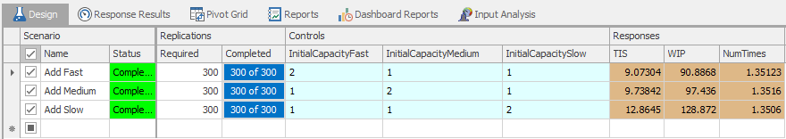
Figure 5.38: Experiment Design for Model 5-4 showing the referenced properties and results.
Three aspects of our experiment warrant discussion at this point – the Controls and Responses (columns in the experiment table) and the Scenarios (rows in the experiment table). We introduced experiment Responses in Section 4.5, where we demonstrated how responses are used in Simio MORE (SMORE) plots. In Model 5-4, we’ve defined the following responses:
- TIS (Time in System): The time that an average entity (PCB) spends in the system. Simio tracks this statistic automatically for each entity type (
PCB.Population.TimeInSystem.Averagefor the PCB objects). - WIP (Work in Process): The average number of entities (PCBs) in the system. Simio also tracks this statistic automatically for each entity type (
PCB.Population.NumberInSystem.Averagefor the PCB objects). - Num Times: The average number of times that an entity is processed by the placement machine. We defined the corresponding tally statistic in Section 5.3.1 and use the expression
NumTimesProcessed.Averageto access the average value.
You can see in Figure 5.38 that the current response values are displayed as the experiment runs. The controls columns include the referenced properties that we created and used to specify the initial capacities of the three fine-pitch placement machine objects. In an experiment, the values for these properties can be set, and we can define a scenario by specifying the number of replications to run and values for each of the three referenced properties. As shown in Figure 5.38, we’ve defined three scenarios using the referenced properties to define the configurations — one for adding a fast machine, one for adding a medium machine, and one for adding a slow machine (and named accordingly). With multiple scenarios, you can explicitly control which ones Simio runs by checking/unchecking the boxes in the far left column of the experiment table. Depending on your computer processor type, Simio will run one or more scenarios simultaneously.
Figure 5.39 shows the Response Chart tab (the SMORE plot, introduced in Section 4.5) for our 3-scenario experiment with the TIS response selected. Note that the three SMORE plots are displayed on the same scale allowing a direct comparison. For these SMORE plots, we specified the Upper Percentile as 90% and the Lower Percentile as 10%, so the box in the box plot contains the middle 80% of the responses from the 300 replications; we also opted to display the plots with the value axes’ being horizontal, via the Rotate Plot button in the Response Chart ribbon. As we might expect, the Add Fast scenario appears to be better (smaller average times in system) than the other two, and Add Medium appears better than Add Slow; you’ll find a similar pattern with the WIP Responses selected from the pull-down near the top left of the chart (not shown).
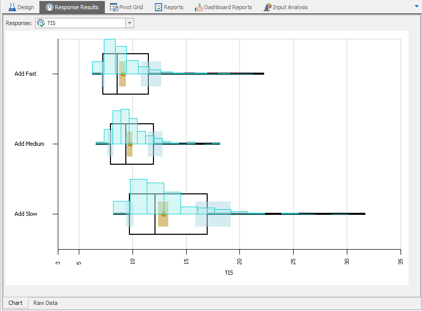
Figure 5.39: SMORE plot for the average-time-in-system Response in Model 5-4.
Figure 5.40 shows the SMORE plot for the average number of times that an entity is processed by the placement machine (the NumTimes Response). As we’d expect, the number of times that a board is processed does not appear to depend on whether we buy a fast, medium, or slow fine-pitch placement machine.
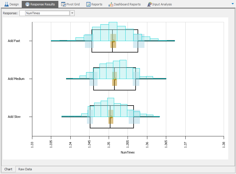
Figure 5.40: SMORE plot for the NumTimes Response in Model 5-4.
While some scenarios may appear better than others in the SMORE plots for TIS and WIP, we must be careful to use statistically valid comparisons before drawing formal conclusions. One route to this might be to use Simio’s Export Details capability (discussed in Section 4.6) to create a CSV file with each response from each replication, and then import that into a dedicated statistical-analysis package that will provide several statistical-comparison methods. One such method, if we’re interested in comparing means, is the classical paired-\(t\) approach to building a confidence interval on the difference between means of two scenarios, or doing hypothesis tests on the difference between two means. Here, we use the paired-\(t\) approach, rather than the two-sample-\(t\) approach, since the same underlying random numbers are used to run all scenarios, so they are not independent. The paired approach can tolerate this non-independence, but the two-sample approach requires independent samples, so separate random numbers across all scenarios. Note that this allows only two scenarios to be compared at a time, so in a situation like ours with more than two scenarios, we could perhaps do all pairwise comparisons (Fast vs. Medium, then Fast vs. Slow, then Medium vs. Slow), but we need to remember that the overall confidence level degrades when doing multiple statistical comparisons in this way. Alternatively, methods like analysis of variance (ANOVA) could be used to compare all the means at once, with standard post-test multiple-comparison methods (Tukey, Scheffe, Bonferroni, etc.) For details, see any standard statistics text.
Since this situation of comparing multiple alternative scenarios is quite common in simulation applications, special statistical methods have been developed for it. If you look back carefully at the TIS and WIP response columns in Figure 5.38, you’ll notice that the Response values for the Add Medium and Add Slow scenarios are shaded light brown, but are shaded darker brown for the Add Fast scenario. This is a result of the Subset Selection Analysis available in Simio Experiments, which uses sound statistical methods from (Boesel, Nelson, and Kim 2003) to divide the scenarios into two subsets in terms of their estimated mean responses, “possible best” (shaded the darker brown) and “rejects” (shaded the light brown), based on the 300 replications that were already run for each scenario. The essential interpretation of this, per (B. L. Nelson 2013), is that “everything in the [possible-best] subset is statistically indistinguishable from the sample best” in terms of sample means. To make this Subset Selection happen, after completing your Experiment runs, first select the TIS response in the Experiment Design window, and in the resulting Properties grid under Objective, select Minimize (via the pull-down at the right) since smaller values for average time in system are better. Then, in the ribbon for the Experiment Design, click on the Subset Selection icon in the Analysis section, and the algorithm decides which scenarios are “possible best” (Add Fast, which is shaded the darker brown), and which are “rejects” (Add Medium and Add Slow, which are shaded the light brown). You should choose the overall statistical confidence level for this conclusion in the Experiment Properties under Confidence Level to be 90%, 95%, 98%, or 99%. You can repeat all this for the WIP Responses, where smaller is once again better, so you would again choose Minimize for the Objective property; we’d actually done this, and happened to get the same subsets of “possible best” and “rejects” as we did for the TIS responses, though such agreement for all responses is generally not to be expected. (We did not do Subset Selection for the NumTimes Responses since it’s not clear whether we “want” this to be big or small.)
In Subset Selection, things don’t always work out as conclusively as they did in this example, since the subset of “possible best” scenarios could contain more (maybe a lot more) than just a single scenario. In such a case, Simio provides an Add-In, Select Best Scenario using KN, available under the Select Add-In icon on the Experiment ribbon, to narrow things down for you; again, this is based on means. Using algorithms in (Kim and Nelson 2001), this add-in commandeers your Experiment run, sequentially increasing the number of replications for some scenarios as called for by the algorithm, in order to isolate one scenario as very likely “the best,” based on the Response you select (only one Response at a time can be considered). You must provide a confidence level for this selection, and an indifference zone (a value small enough so that you don’t care if the mean of your selection is inferior to the mean of the true best scenario by this amount or less), as well as a replication limit that you might set based on your initial experimentation with the model. For more information on how this procedure works in Simio, see the Simio Reference Guide topic “Select Best Scenario Using KN Add-In,” and of course (Kim and Nelson 2001) for the underlying methods; in Section 9.1.2 we use this KN Add-In to select the best scenario in a larger example.
5.6 Summary
In this chapter we’ve moved things along into intermediate modeling with several new Simio concepts, building on a firmer foundation of how the object orientation of Simio is defined. We also have discussed how to do a sound statistical analysis when comparing multiple alternate simulated scenarios. All of this provides a solid basis for further study of simulation with Simio, including model data, animation, and advanced modeling techniques, to be covered in the chapters that follow.
5.7 Problems
- What is the difference between an object property and an object state?
- Consider a process associated with a Server object. What is the difference between a token’s parent object and it’s associated object?
- Develop a queueing model that gives the steady-state values analogous to the values in Table 5.2 (Model 5-1 with exponential processing times at both stations).
- Consider an office where people come to get their drivers’ licenses. The process involves three steps for arriving customers — reception / application; a vision exam; and a written exam. Assume that customer arrivals are Poisson with a rate of 6 per hour (i.e., interarrival times are exponentially distributed with mean 10 minutes). The processing time distributions for the three processes are given in Table 5.8. The office has one person responsible for reception/application and one person responsible for administering the vision exams. The written exam is computer-based and there are three computer stations where customers can take the exam. Develop a Simio model of this system. Assume that the office opens at 9:00 a.m. and closes at 5:00 p.m. The performance metrics of interest include the time that customers spend in the system, the utilizations of the office employees and the computer stations, and the average and maximum numbers of customers in the reception/application queue, the vision exam queue, and the written exam queue. How many replications should be run in order to be confident about your results? Justify your answer.
- Animate the model from Problem 4. If you did not already do so, specify a reasonable office layout and use Path object to incorporate customer movement through the office. Make sure that the distances between stations are reasonable for a drivers’ license office and that the entity speed is appropriate for humans walking.
- In Model 5-2, we assumed that the inspection workers did not overlap between shifts (i.e., there were never two inspectors working at the same time). Modify the model so that the inspectors do overlap for the first hour of one shift and the last hour of the other shift. Compare the results of the two models. Does having the inspectors overlap help?
- In the description of Model 5-2, we noted that there is no limit on the number of times that a board may be found in need of rework. Modify Model 5-2 so that if a board fails the inspection more than two times, it is rejected as a bad part. Count the number of boards that are rejected because of 3 or more failures of inspection.
- In the description of Model 5-3, we indicated that as part of our model verification, we had predicated the proportions of parts that would go to the fast, medium and slow fine-pitch placement machines (38%, 33%, and 29%, respectively). Develop a queueing model to estimate these proportions.
- Consider a pharmacy where customers come to have prescriptions filled. Customers can either have their doctor fax their prescriptions ahead of time and come at a later time to pick up their prescriptions or they can walk in with the prescriptions and wait for them to be filled. Fax-in prescriptions are handled directly by a pharmacist who fills the prescriptions and leaves the filled prescriptions in a bin behind the counter. Tip: This solution makes use of two basic Rate Tables which are covered in Section 7.3 if you are not already familiar with the concepts.
- Historical records show that approximately 59% of customers have faxed their prescriptions ahead of time and the times for a pharmacist to fill a prescription are triangularly distributed with parameters (2,5,8) minutes. If an arriving customer has faxed his/her prescription in already, a cashier retrieves the filled prescription from the bin and processes the customer’s payment. Historical records also indicate that the times required for the cashier to retrieve the prescriptions and process payment are triangularly distributed with parameters (2,4,6) minutes. If an arriving customer has not faxed the prescription ahead of time, the cashier processes payment and sends the prescription to a pharmacist, who fills the prescription. The distributions of the cashier times and pharmacist times are the same as for the fax-in customers (triangular(2,4,6) and triangular(2,5,8), respectively). Fax-in and customer arrival rates vary during the day as do the pharmacy staffing levels. Table 5.9 gives the arrival and staffing data where \(C\) is the number of cashiers, \(P\) is the number of Pharmacists, \(\lambda_1\) is the arrival rate for fax-in prescriptions and \(\lambda_2\) is the arrival rate for customers.
- Develop a Simio model of this pharmacy. Performance metrics of interest include the average time fax-in prescriptions take to be filled, the average time customers spend in the system, and the scheduled utilizations of the cashiers and pharmacists. Assume that the pharmacy opens at 8:00 a.m. and closes at 10:00 p.m. and you can ignore faxes and customers that are still in the system at closing time (probably not the best customer service!). Use 500 replications for your analysis and generate the SMORE plots for the performance metrics of interest.
- Develop a Simio model of the serial manufacturing system shown in Figure 5.41. Assume that parts arrive to the system at the rate of 120 per hour and that the arrivals are Poisson. The characteristics of each machine are given in Table 5.10.
Your model should include the following characteristics/features:
- Parts (entities) should move from machine to machine instantaneously (0 simulated time).
- Name the object instances in your model using meaningful names.
- Create a user-defined statistic that tracks the number of “reworks” in the system, where a “rework” is any part that has been reworked at least once (i.e., it’s entered S1 more than once).
- Create a status plot that displays (1) the instantaneous number of entities in the system, (2) the average number of entities in the system, and (3) the instantaneous number of reworks in the system (see above). The time range for the plot should be 25 hours.
- Develop an interesting animation for your model.
- Create an experiment with the following conditions:
- Run length — 200 hours;
- Warmup — 50 hours;
- 20 replications.
- Create experiment responses for each of the following:
- Average number of parts in the system;
- Maximum number of reworks in the system;
- Average time (in minutes) that parts spend in the system;
- The utilization of S4;
- The rate at which good parts are finished (in parts per hour);
- The rate at which parts fall-out from S3 (in parts per hour).
| Process | Processing time distribution |
|---|---|
| Reception/application | triangular(5, 8, 11) |
| Vision exam | triangular(2, 4, 6) |
| Written exam | triangular(10, 15, 20) |
| Time Period | \(C\) | \(P\) | \(\lambda_1\) | \(\lambda_2\) |
|---|---|---|---|---|
| 8:00 a.m. - 11:00 a.m. | 1 | 2 | 10 | 12 |
| 11:00 a.m. - 3:00 p.m. | 2 | 3 | 10 | 20 |
| 3:00 p.m. - 7:00 p.m. | 2 | 2 | 10 | 15 |
| 7:00 p.m. - 10:00 p.m. | 1 | 1 | 5 | 12 |
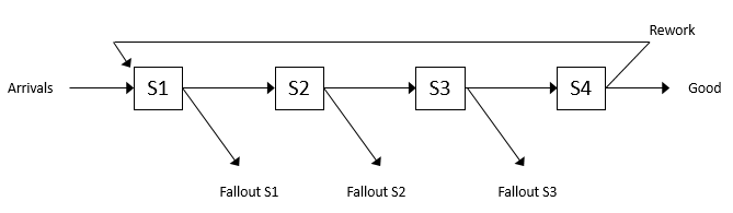
Figure 5.41: Serial manufacturing system for Problem 10.
| S1 | S2 | S3 | S4 | |
|---|---|---|---|---|
| ST (secs) | unif(10, 20) | tria(20, 30, 40) | unif(60, 84) | expo(40) |
| Servers (c) | 1 | 1 | 2 | 1 |
| F/R prob. | 0.15 | 0.30 | 0.33 | 0.08 |