Simio and Simulation: Modeling, Analysis, Applications - 7th Edition
Chapter 12 Simulation-based Scheduling in Industry 4.0
As discussed in Chapter 1, and illustrated throughout the book, simulation has been used primarily to enhance the design of a system — to compare alternatives, optimize parameters, and predict performance. Although having a good system design is certainly valuable, there is a parallel set of problems in effectively operating a system.
A Smart Factory initiative is here now! Over the last several years the required technology has dramatically improved and is rapidly gaining attention around the world. This approach to running a factory currently has some remaining challenges that can perhaps be best addressed by evolving simulation technology and applying simulation to new applications.
This chapter will begin by discussing the evolution and current state of Industry 4.0 and some of its challenges and opportunities, then discuss ways that simulation can be used within Smart Factories in its more traditional role, as well as within the Digital Twin space. We will explore some of the current technology used for planning and scheduling, and then end with an introduction to Risk-based Planning and Scheduling (RPS). Some material in this chapter is similar to that found on the Simio web site and is included with permission (LLC 2018).
12.1 Industrial Revolutions through the Ages
Industry 4.0 is the common name used to describe the current trend towards a fully connected and automated manufacturing system. “We stand on the brink of a technological revolution that will fundamentally alter the way we live, work and relate to one another,” (Schwab 2017) said Klaus Schwab, the Founder and Executive Chairman of the World Economic Forum in his book The Fourth Industrial Revolution. This statement was made at the beginning of 2017 but could just as well have been said 200 years ago, before the first industrial revolution redefined civilization.
Before we discuss Industry 4.0, let’s take a brief look at the stages that brought us to where we are today (Figure 12.1).
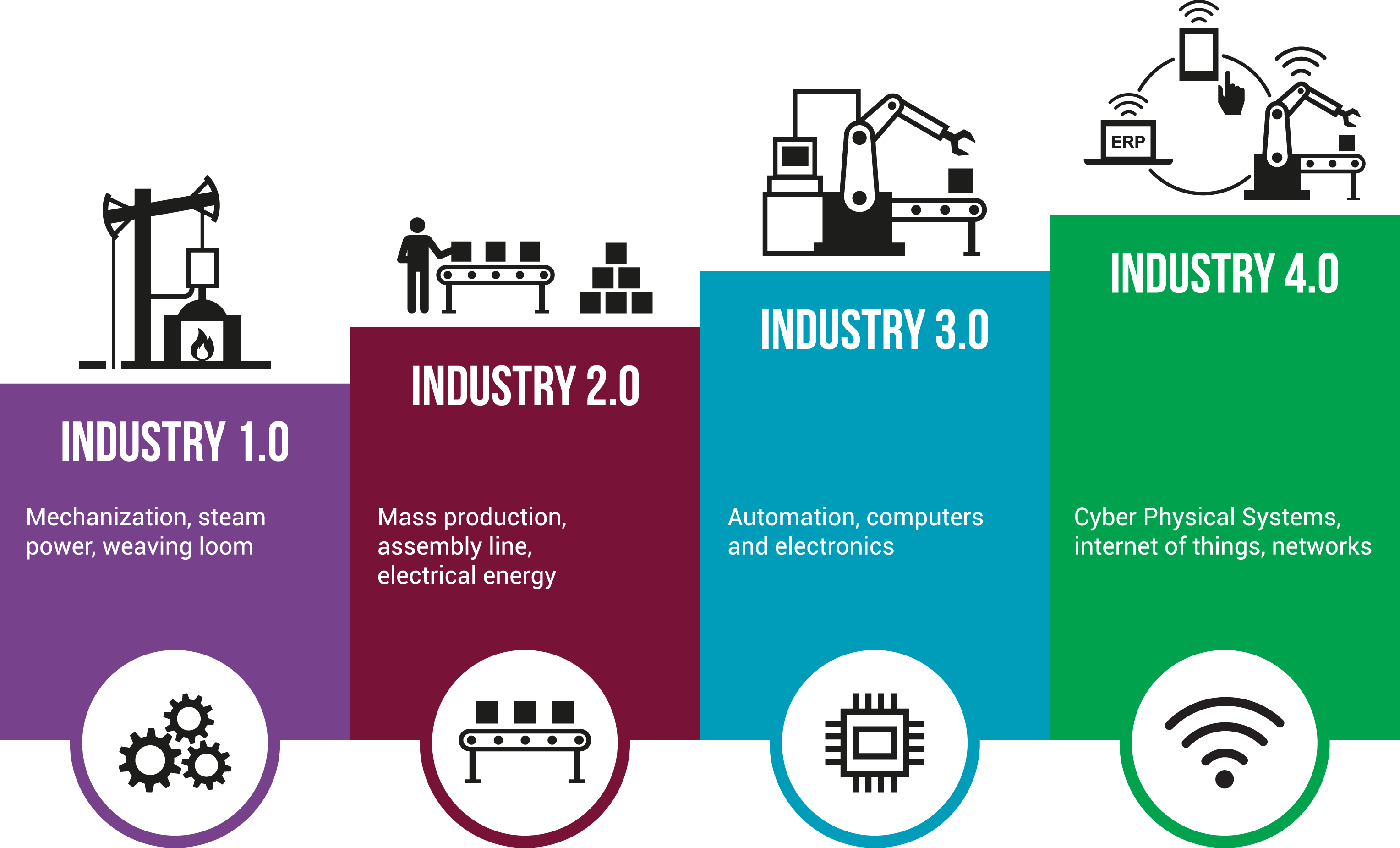
Figure 12.1: History of industrial revolutions.
12.1.1 First Industrial Revolution – Mechanical Production
Prior to 1760, the world’s population was totally insular, living in closed communities with limited skill sets and food supplies, following family traditions, with no thought of change. Starting in the United Kingdom, with the invention and refinement of the steam engine and steam power, agriculture boomed and food supplies fueled increases in population, leading to the development of new markets.
Allowing factories to spring up anywhere, not just around water mills, industrialization spread. Cities were created, full of consumers and the growth of the railroads allowed even further expansion and urbanization. Agriculture was abandoned in favor of the production of goods in the forms of textiles, steel, food, and more. Jobs were created, areas such as the media, transport systems, and medical services were reinvented, and everyday life was transformed.
All this took place over a period of around 80 years, until the mid-1800s, its effect spreading out into Europe and the Americas.
12.1.2 Second Industrial Revolution – Mass Production
As the 20th century dawned, population and urbanization continued to grow, boosted massively by the latest invention and widespread use of electrical power. The 2nd industrial revolution sparked developments into mass production with assembly lines for food, clothes and goods, as well as major leaps forward in transport, medicine, and weapons.
Europe remained dominant, but other nations were now attaining the power and technology to advance independently.
12.1.3 Third Industrial Revolution – The Digital Age
By the 1960s, civilization had settled down again after two World Wars, with new applications of wartime technology sparking innovation and forward thinking once again in peacetime. The usefulness of the silicon wafer was discovered, leading to the development of semiconductors and mainframe computers, evolving into personal computers in the 1970s and 1980s. With the growth of the internet in the 1990s, the computer, or digital, revolution was internationally well underway.
12.2 The Fourth Industrial Revolution – The Smart Factory
The Fourth Industrial Revolution is said to be the biggest growth leap in human history adding a whopping 10 to 15 trillion dollars to global GDP over the next 20 years (Components 2015). Conceived in Germany, Industry 4.0 is also known as Industrie 4.0, Smart Factory, or Smart Manufacturing. It is so named because of its huge impact in the way companies will design, manufacture, and support their products. Manufacturing has once again provided the growth impetus for this new phenomenon, with the merging of the virtual and physical worlds. Having implemented ideas to reduce labor costs and improve manufacturing productivity, the natural next step is the application of technology for the digital transformation of manufacturing. In this fully connected and automated manufacturing system, production decisions are optimized based on real-time information from a fully integrated and linked set of equipment and people.
Existing digital industry technologies encompassed by Industry 4.0 include:
Internet of Things (IoT) and Industrial Internet of Things (IIoT)
Robotics
Cloud Computing/Software as a Service (SaaS)
Big Data/Advanced Analytics
Additive Manufacturing/3D Printing
System Integration
Augmented/Virtual Reality (VR)
Simulation
IT/Cybersecurity
Industry 4.0 embraces and combines these technologies to facilitate massive process improvement and productivity optimization. The resulting innovation will eventually lead to the development of radical new business models that have their foundations in Information and Services. For most manufacturers, Industry 4.0 is currently only a vision to strive for, however, digital transformation of the industry is already underway with the use of advanced manufacturing robots and 3D printing, now impacting on the realms of both plastics and metals. Potential benefits and improvements are already being realized in production flexibility, quality, safety and speed. Equally, new challenges are arising, especially in the fields of information management, production scheduling and cyber security.
Already reaching beyond its original intended scope, Industry 4.0 is bringing about a new era, with the ability to manufacture batches consisting of single items, or of thousands, each having the same lead times and costs. A huge macroeconomic shift is coming that will see smaller, more agile factories existing nearer the consumer to facilitate regional trade flows.
Since Industry 4.0 can be applied to the entire product life cycle and value chain, it can affect all stakeholders; however, its success depends upon effective information flow throughout the system. This is where the benefits of cutting-edge simulation and scheduling software become critically important for data collection, planning and scheduling.
12.2.1 What’s Next?
Speed and momentum gathered as new discoveries continued to be made through collaboration and knowledge sharing, leading to where we are now. Building on the digital revolution, we now have the far-reaching mobile internet, inexpensive solid state memory capabilities, and massive computing power resources. Combined with smaller, more powerful devices and sensors, we are now able to draw on information to advance even further, using technologies such as robotics, big data, simulation, machine learning, and artificial intelligence.
Smart factories allow cooperation between these virtual and physical systems, allowing the creation of new operating models that can even be represented as Digital Twins for diagnostic and productivity improvement. There is still work to be done in fulfilling these opportunities and turning potential solutions into efficient solutions.
Beyond that, we are anticipating great leaps forward in fields such as nanotechnology, renewables, genetics and quantum computing, now linking the physical and digital domains with biological aspects in a new branch of this latest revolution. The speed of change is astounding, compared to the long, slow spread of those first revolutionary developments. Technology is moving so quickly, with globally connected devices making the world even smaller, allowing exchanges of skills and ideas to propagate new inventions across disciplines.
Without the small first step of the 1st Industrial Revolution, however, we would be continuing our insular lives with no travel or exploration, limited food sources, susceptibility to health challenges and no prospect of innovation. So, although we are now continually on the brink of profound change and momentous international developments are becoming inevitable, we need to embrace those developments and open our imaginations to move forward on this exciting step of our course in history.
As Klaus Schwab concluded; “In its scale, scope, and complexity, the transformation will be unlike anything humankind has experienced before.” (Schwab 2017)
12.3 The Need for a Digital Twin
In the consumer environment, the Internet of Things (IoT) provides a network of connected devices, all with secure data communication to allow them to work together cooperatively. In the manufacturing environment, the Industrial Internet of Things (IIoT) allows the machines and products within the process to communicate with each other to achieve the end goal of efficient production. With the growing move toward Industry 4.0, increased digitalization is bringing its own unique challenges and concerns to manufacturing. One way of meeting those challenges is with the use of a Digital Twin.
A Digital Twin provides a virtual representation of a product, part, system, or process that allows you to see how it will perform, sometimes even before it exists. Sometimes this term is applied at the device level. A digital twin of a device will perform in a virtual world very similar to how the real device performs in the physical world. An important application is a digital twin of the entire manufacturing facility that again performs in a virtual world very similar to how the entire manufacturing facility performs in the physical world. The latter, broader definition of a digital twin may seem unattainable, but it is not. Just like in the design-oriented models we have already discussed, our objective is not to create a “perfect model” but rather to create a model that is “close enough” to generate results useful in meeting our objectives. Let’s explore how we can meet that goal.
According to some practitioners, you can call a model a digital twin only when it is fully connected to all the other systems containing the data to enable the digital twin. A standalone simulation model will be referred to as a virtual factory model but not a digital twin until it is fully connected and runs in real-time (near real-time) mode, driven by data from the relevant ERP, MES, etc. systems. It is therefore also important that you should be able to generate models from data as introduced in Section 7.8 to function effectively as a digital twin. This allows the model to react based on the changes in data – items like adding a resource/machine and having that automatically created in the model and schedules, by just importing the latest data.
In the current age of Industry 4.0, the exponential growth of technological developments allows us to gather, store, and manipulate data like never before. Smaller sensors, cheaper memory storage and faster processors, all wirelessly connected to the network, facilitate dynamic simulation and modeling in order to project the object into the digital world. This virtual model is then able to receive operational, historical and environmental data.
Technological advancements have made the collection and sharing of large volumes of data much easier, as well as facilitating its application to the model, and evaluating various possible scenarios to predict and drive outcomes. Of course, data security is an ever-important consideration with a Data Twin, as with any digital modeling of critical resources. As a computerized version of a physical asset, the Digital Twin can be used for various valuable purposes. It can determine its remaining useful life, predict breakdowns, project performance and estimate financial returns. Using this data, design, manufacturing, and operation can be optimized in order to benefit from potential opportunities.
There is a three stage process to implement a useful Digital Twin:
Establish the model. More than just overlaying digital data on a physical item, the subject is simulated using 3D software. Interactions then take place with the model to communicate with it about all the relevant parameters. Data is imposed and the model “learns”, through similarity, how it is supposed to behave.
Make the model active. By running simulations, the model continuously updates itself according to the data, both known and imposed. Taking information from other sources including history, other models, connected devices, forecasts and costs, the software runs permutations of options to provide insights, relative to risk and confidence levels.
Learn from the model. Using the resulting prescriptions, plans can be implemented to manipulate the situation to achieve optimal outcomes in terms of utilization, costs, and performance, and avoid potential problem areas or unprofitable situations.
A Digital Twin is more than just a blueprint or schematic of a device or system; it is an actual virtual representation of all the elements involved in its operation, including how these elements dynamically interact with each other and their environment. The great benefits come through monitoring these elements, improving diagnostics and prognostics, and investigating root causes of any issues in order to increase efficiencies and overall productivity.
A correctly generated Digital Twin can be used to dynamically calibrate the operational environment in order to positively impact every phase of the product lifecycle; through design, building and operation. For any such application, before the digital twin model is created, the objectives and expectations must be well understood. Only then can a model be created at the correct fidelity to meet those objectives and provide the intended benefits. Examples of those benefits include:
Equipment monitors its own state and can even schedule maintenance and order replacement parts when required.
Mixed model production can be loaded and scheduled to maximize equipment usage without compromising delivery times.
Fast rescheduling in the event of resource changes reduces losses by re-optimizing loading to meet important delivery dates.
12.4 Role of Design Simulation in Industry 4.0
For decades, simulation has been used primarily for facility design improvements. Section 1.2 lists some of the many application domains where simulation is routinely used, often for purposes like:
Supply Chain Logistics: Just-in-time, risk reduction, reorder points, production allocation, inventory positioning, contingency planning, routing evaluations, information flow and data modeling
Transportation: Material transfer, labor transportation, vehicle dispatching, traffic management (trains, vessels, trucks, cranes, and lift trucks)
Staffing: Skill-level assessment, staffing levels and allocation, training plans, scheduling algorithms
Capital investments: Investing for growth. Determining the right investments, at the right time. Objective evaluation of return on investment
Productivity: Line optimization, product-mix changes, equipment allocation, labor reduction, capacity planning, predictive maintenance, variability analysis, decentralized decision-making
The first answer to how simulation can assist with Industry 4.0 is “all of the above”. At its simplest, a smart factory is just a factory – it has all the same problems as any other factory. Simulation can provide all of the same benefits in the same areas where simulation has traditionally been used. In general, simulation can be used to objectively evaluate the system and provide insight into its optimal configuration and operation.
Of course, a smart factory implementation is much more than “just a factory” and differs in many important ways. First of all, a smart factory is generally larger and has not only more components, but more sophisticated components. While an optimist might read “sophisticated” as “problem free”, a pessimist might read that as “many more opportunities to fail”. Either way, a larger system with more interactions is harder to analyze and makes the traditional application of simulation even more important. It is difficult to assess the impact of any specific advanced feature. Simulation is possibly the only tool to allow you to objectively evaluate the interactions and contributions of each component, design a system that will work together, and then tune and optimize that system.
In a smart factory, IT innovations such as big data and cloud operation make real time data much more available. Although effectively handling large amounts of data is not a strength of all simulation products, more modern products allow incorporating such data into a model. While this enhanced data access potentially enables the system to perform better, it also exposes still more points of failure and the opportunity for a model of sufficient detail to identify areas of risk before implementation.
Another way that a smart factory differs is its level of automation and autonomy. The dynamic processes in a smart factory enable operational flexibility, such as intelligently responding to system failures and automatically taking corrective action, both to correct the failure and to work around the failure with appropriate routing changes. Simulation can help assess those actions by evaluating the performance of alternatives. Just as in a normal factory, a smart factory can’t readily be run over and over with different configurations and settings. Simulation is designed to do just that. It effectively projects future operations, compressing days into just seconds. Further, the simulation model can be easily adjusted when the effects of scaling up or down the system need to be studied. The resulting information answers fundamental questions about the processes and overall system. For example, how long a process takes, how frequently some equipment is used, how often rejects appear, etc. Consequently, it predicts performance criteria such as latency, utilization and bottlenecks for direct improvement.
A large benefit for larger organizations using this virtual factory model is standardization of data, systems, and processes. Typically each factory within a large corporation has implemented their systems differently. These differences cause big problems when moving these facilities to single instances of ERP. People need to be using the same processes and workflows, but how do they decide what process is the best and what data is correct or preferable? Using the virtual factory model to test different operational policies and data is the best way to determine the single best global process and adjust all factories accordingly. Using simulation with a data generated approach, is valuable and interesting to these large corporations with multiple global factories.
Two other benefits of simulation are particulary applicable to smart factories – establishing a knowledgebase and aiding communication. It is very difficult to describe how a complex system works, and perhaps even more difficult to understand it. Creation of a model requires understanding how each subsystem works and then representing that knowledge in the model. The simulation model itself becomes a repository of that knowledge - both direct knowledge embedded in its components and indirect knowledge that results from running the model. Likewise, the 2D or 3D model animation can be an invaluable way of understanding the system so stakeholders can better understand how the system works, more effectively participate in problem resolution, and hence have better buy-in to the results.
Although time consuming, the modeling stage requires the involvement of operators and personnel who are intimately familiar with the processes. This involvement imparts an immediate sense of ownership that can help in the later stage when implementing findings. To that end, a realistic simulation proves to be a much easier and faster tool than alternatives like spreadsheets, for testing and understanding performance improvements in the context of the overall system. This is especially true when demonstrating to users and decision makers.
In these ways, simulation assists with:
predicting the resulting system performance,
discovering how the various parts of the system interact,
tracking statistics to measure and compare performance,
providing a knowledgebase of system configuration and its overall performance, and
serving as a valuable communication tool.
In summary, use of simulation in its traditional design role can provide a strong competitive advantage during development, deployment and execution of a smart factory. It can yield a system that can be deployed in less time, with fewer problems, and yield a faster path to optimal profitability.
12.5 The Role of Simulation-based Scheduling
The rise of Industry 4.0 has expedited the need for simulation of the day-to-day scheduling of complex systems with expensive and competing resources. This operational need has extended the value of simulation beyond its traditional role of improving system design into the realms of providing faster, more efficient process management, and increased performance productivity. With the latest technologies, like Risk-based Planning and Scheduling (RPS), the same model that was built for evaluating and generating the design of the system can be carried forward to become an important business tool in scheduling day-to-day operations in the Industry 4.0 environment.
With digitalized manufacturing, connected technologies now form the smart factory, having the ability to transmit data to help with process analysis and control during the production process. Sensors and microchips are added to machines, tools, and even to the products themselves. This technology allows ‘smart’ products made in the Industry 4.0 factory to transmit status reports throughout their journey, from raw material to finished product.
Increased data availability throughout the manufacturing process means greater flexibility and responsiveness, making the move towards smaller batch sizes and make-to-order possible.
In order to capitalize on this adaptivity, an Industry 4.0 scheduling system needs to:
accurately model all elements,
compute schedules quickly,
provide easy visualization.
With IoT devices, big data and cloud computing as features of Industry 4.0, the scheduling system needs more than ever to bridge the gap between the physical and digital worlds.
Traditionally, there are three approaches to scheduling: manual, constraint-based, and simulation.
Labor-intensive, manual scheduling, often using tools like white boards and spreadsheets, can be effective in smaller or less complex systems. But, as the name implies, a manual approach relies heavily on a person’s ability to understand all the relationships and possible alternatives. Such an approach becomes impractical in a large, highly dynamic production environment, due to the sheer volume and complexity of data.
Constraint-based scheduling involves the solution of equations that are formulated to represent all of the system constraints. A mathematical model could be built of all the elements of a smart factory; however, it would be highly complicated to populate and solve, probably taking a long time to do so. Key aspects would have to be ignored or simplified to allow for a solution which, when found, would be difficult to interpret, visualize and implement.
For both manual and constraint-based scheduling, often scheduling is done for a single department or section of the facility to reduce complexity. These localized schedules often require process buffers between sections, wasting a combination of time, inventory, or capacity.
Simulation-based scheduling stands out as the best solution for Industry 4.0 applications. Each element of the system can be modeled and data assigned to it. The resources (i.e., equipment, tools, and workers) can be represented, as well as the materials consumed and produced in the process. In this way, the flow of jobs through the system can be simulated, showing exact resource and material usage at each stage, and providing real-time status updates.
Decision logic can be embedded in the model, for example, to select minimum changeover times, as well as custom rules added from worker experience. These algorithms combine to produce a range of rules that accurately model the actual flow of materials and components through the system.
This technology allows simulation-based scheduling software to perform calculations and permutations on all aspects of the production process. This ability, combined with the large volume of real-time data provided by the digitalized workstations, means that scheduling is fast, detailed, and accurate.
Three main requirements for scheduling in Smart factories are satisfied by simulation-based scheduling software:
Accurate modeling of all elements – a flexible model is generated from computerized information, including full representation of operating constraints and custom rules.
Fast computation of schedules – calculation of schedules and scheduling alternatives, comparison and distribution is carried out quickly and precisely.
Easily visualized – computerized simulation allows the schedule to be communicated clearly and effectively across all organizational levels.
Improved labor effectiveness is another benefit of simulation-based scheduling. The details generated enables the use of technology like “smart glass” which may be one of the most significant ways of enabling the labor force – smart glasses will provide employees with timely, detailed instructions. By constantly evaluating the schedule, the simulation model will use actual and current data to direct each worker to the most efficient way to perform the next task.
While such a schedule is an essential part of a smart factory, the model can actually play an even more integral role than just scheduling as we see in the next section.
12.5.1 Simulation as the Digital Twin
The IT innovations of Industry 4.0 allow data collected from its digitalized component systems in the smart factory to be used to simulate the whole production line using Discrete Event Simulation software. Real-time information on inventory levels, component histories, expiration dates, transport, logistics and much more can be fed into the model, developing different plans and schedules through simulation. Alternative sources of supply or production plans can be evaluated against each other while minimizing potential loss and disruption.
When change happens, be it a simple stock out or equipment breakdown, or a large scale natural disaster, simulation models can show the impact on production and how downstream services will be affected and. Revised courses of action can then be manually or automatically assessed and a solution implemented.
The benefits of using simulation to schedule and reduce risk in an Industry 4.0 environment include assuring consistent production, where costs are controlled and quality is maintained given any circumstances. By leveraging scheduling, highly data-driven simulation models can also fill the role of a Digital Twin. Figure 12.2 illustrates how a simulation model can sit at the core of a smart factory. It can communicate with all of the critical sub-systems, collect planning and real-time execution information, automatically create a short-term schedule, and distribute the components and results of that schedule back to each sub-system for further action.
Figure 12.2: Digital twin enabling the smart factory.
Advanced simulation-based scheduling software is uniquely suited for such an application due to its:
ability to communicate in batch or real-time with any sub-system,
model the complex behavior required to represent the factory,
execute sophisticated techniques to generate a suitably optimal schedule,
report that schedule back to stakeholders for execution,
then wait for a deviation from plan to be reported which could cause a repeat of the process.
This fills an important gap left in most smart factory plans.
12.6 Tough Problems in Planning and Scheduling
Planning and scheduling are often discussed together because they are related applications. Planning is the “big-picture” analysis – how much can or should be made, when, where, and how, and what materials and resources will be required to make it? Planning is typically done on an aggregate view of the capacity assuming infinite material. Scheduling is concerned with the operational details – given the current production situation, actual capacities, resource availabilities, and work in progress (WIP), what priorities, sequencing, and tactical decisions will result in best meeting the important goals? Where planning is required days, weeks or months ahead of execution, scheduling is often done only minutes, hours, or days ahead. In many applications, planning and scheduling tasks are done separately. In fact, it is not unusual for only one to be done while the other may be ignored, leaving significant unrealized potential performance.
One simple type of planning is based on lead times. For example, if averages have historically indicated that most parts of a certain type are “normally” shipped 3 weeks after an order is released, it will be assumed that — regardless of other factors — when we want to produce one, we should allow 3 weeks. This often does not adequately account for resource utilization. If you have more parts in process than “normal,” the lead times may be optimistic because it may actually take much longer than predicted.
Another simple type of planning uses a magnetic board, white board, or a spreadsheet to manually create a Gantt chart to show how parts move through the system and how resources are utilized. This can be a very labor-intensive operation, and the quality of the resulting plans may be highly variable, depending on the complexity of the system and the experience level of the planners.
A third planning option is a purpose-built system - a system that is designed and developed using custom algorithms usually expressed in a programming language. These are highly customized to a particular domain and a particular system. Although they have the potential to perform quite well, they often have a very high cost and implementation time and low opportunity for reuse because of the level of customization.
One of the most popular general techniques is Advanced Planning and Scheduling (APS). APS is a process that allocates production capacity, resources, and materials optimally to meet production demand. There are a number of APS products on the market designed to integrate detailed production scheduling into the overall Enterprise Resource Planning (ERP) solution, but these solutions have some widely recognized shortcomings. For the most part the ERP system and day-to-day production remain disconnected largely due to two limitations that impede their success: complexity and variation.
Complexity. The first limitation is the inability to effectively deal with indeterminately complex systems. Although purpose-built systems can potentially represent any system, the cost and time required to create a detailed, custom-built system often prevents it from being a practical solution. Techniques such as those discussed above tend to work well if the system is very close to a standard benchmark implementation, but to the extent the system varies from that benchmark, the tool may lack enough detail to provide an adequate solution. Critical situations that are not handled include complex material handing (e.g., cranes, robotic equipment, transporters, workers), specialized operations and resource allocations (e.g., changeovers, sequence dependent setups, operators), and experience-based decision logic and operating rules (e.g., order priorities, work selection rules, buffering, order sequence).
Variation. A second limitation is the inability to effectively deal with variation within the system. All processing times must be known and all other variability is typically ignored. For example, unpredictable downtimes and machine failures aren’t explicitly accounted for, problems with workers and materials never occur, and other negative events don’t happen. The resulting plan is, by nature, overly optimistic. Figure 12.3. illustrates a typical scheduling output in the form of a Gantt chart, where the green dashed line indicates the slack between the (black) planned completion date and the (gray) due date. Unfortunately, it is difficult to determine if the planned slack is enough. It is common that what starts off as a feasible schedule turns infeasible over time as variation and unplanned events degrade performance. It is normal to have large discrepancies between predicted schedules and actual performance. To protect against delays, the scheduler must buffer with some combination of extra time, inventory, and capacity; all these add cost to the system.
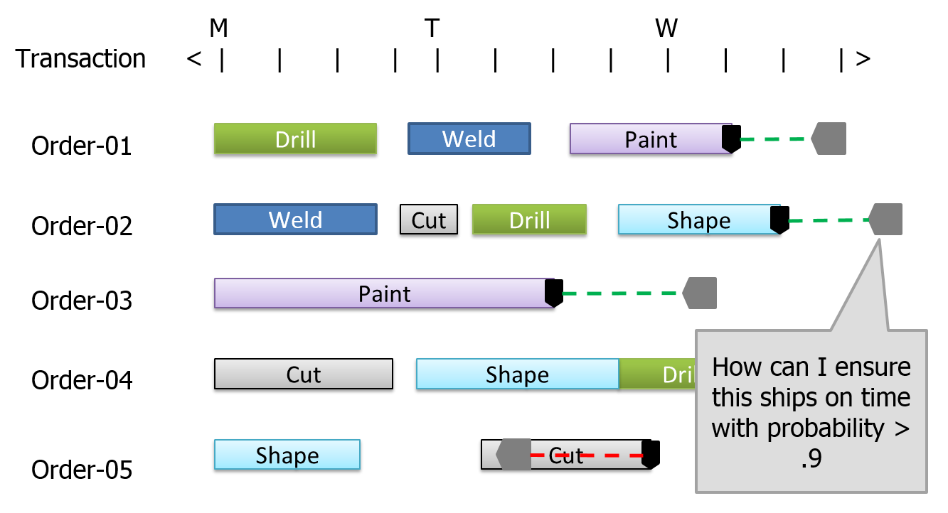
Figure 12.3: Typical Gantt chart produced in planning.
The problem of generating a schedule that is feasible given a limited set of capacitated resources (e.g. workers, machines, transportation devices) is typically referred to as Finite Capacity Scheduling. There are two basic approaches to Finite Capacity Scheduling which will be discussed in this section and the next.
The first approach is a mathematical optimization approach in which the system is defined by a set of mathematical relationships expressed as constraints. An algorithmic solver is then used to find a solution to the mathematical model that satisfies the constraints while striving to meet an objective such as minimizing the number of tardy jobs. Unfortunately, these mathematical models fall into a class of problems referred to as NP-Hard for which there are no known efficient algorithms for finding an optimal solution. Hence, in practice, heuristic solvers must be used that are intended to find a “good” solution as opposed to an optimal solution to the scheduling problem. Two well-known examples of commercial products that use this approach are the ILOG product family (CPLEX) from IBM, and APO-PP/DS from SAP.
The mathematical optimization approach to scheduling has a number of well-known shortcomings. Representing the system by a set of mathematical constraints is a very complex and expensive process, and the mathematical model is difficult to maintain over time as the system changes. In addition, there may be many important constraints in the real system that cannot be accurately modeled using the mathematical constraints and must be ignored. The resulting schedules may satisfy the mathematical model, but are not feasible in the real system. Finally, the solvers used to generate a solution to the mathematical model often take many hours to produce a good candidate schedule. Hence, these schedules are often run overnight or over the weekend. The resulting schedules typically have a short useful life because they are quickly outdated as unplanned events occur (e.g., a machine breaks down, material arrives late, workers call in sick).
This section was not intended as a thorough treatment, but rather a quick overview of a few concepts and common problems. For more in-depth coverage we recommend the excellent text, Factory Physics (Hopp and Spearman 2008).
12.7 Simulation-based Scheduling
The second approach to Finite Capacity Scheduling is based on using a simulation model to capture the limited resources in the system. The concept of using simulation tools as a planning and scheduling aid has been around for decades. One of the authors used simulation to develop a steel-making scheduling system in the early 1980s. In scheduling applications, we initialize the simulation model to the current state of the system and simulate the flow of the actual planned work through the model. To generate the schedule, we must eliminate all variation and unplanned events when executing the simulation.
Simulation-based scheduling generates a heuristic solution – but is able to do so in a fraction of the time required by the optimization approach. The quality of the simulation-based schedule is determined based on the decision logic that allocates limited resources to activities within the model. For example, when a resource such as a machine goes idle, a rule within the model is used to select the next entity for processing. This rule might be a simple static ranking rule such as the highest priority job, or a more complex dynamic selection rule such as a one that minimizes a sequence dependent setup time, or one that selects the job based on urgency by picking the job with the smallest value of the time remaining until the due date, divided by the work time remaining (critical ratio).
Many of the simulation-based scheduling systems have been developed around a data-driven pre-existing, or “canned,” job shop model of the system. For example, the system is viewed as a collection of workstations, where each workstation is broken into a setup, processing, and teardown phase, and each job that moves through the system follows a specific routing from workstation to workstation. The software is configured using data to describe the workstations, materials, and jobs. If the application is a good match for the canned model, it may provide a good solution; if not, there is limited opportunity to customize the model to your needs. You may be forced to ignore critical constraints that exist in the real system but are not included in the canned model.
It is also possible to use a general purpose discrete event simulation (DES) product for Finite Capacity Scheduling. Figure 12.4 illustrates a typical architecture for using a DES engine at the core of a planning and scheduling system. The advantages of this approach include:
It is flexible. A general-purpose tool can model any important aspects of the system, just like in a model built for system design.
It is scalable. Again, similar to simulations for design, it can (and should) be done iteratively. You can solve part of the problem and then start using the solution. Iteratively add model breadth and depth as needed until the model provides the schedule accuracy you desire.
It can leverage previous work. Since the system model required for scheduling is very similar to that which is needed (and hopefully was already used) to fine tune your design, you can extend the use of that design model for planning and scheduling.
It can operate stochastically. Just as design models use stochastic analysis to evaluate system configuration, a planning model can stochastically evaluate work rules and other operational characteristics of a scheduling system. This can result in a “smarter” scheduling system that makes better decisions from the start.
It can be deterministic. You can disable the stochastic capabilities while you generate a deterministic schedule. This will still result in an optimistic schedule as discussed above, but because of the high level of detail possible, this will tend to be more accurate than a schedule based on other tools. And you can evaluate how optimistic it is (see next point).
It can evaluate risk. It can use the built-in stochastic capability to run AFTER the deterministic plan has been generated. By again turning on the variation – all the bad things that are likely to happen - and running multiple replications against that plan, you can evaluate how likely you are to achieve important performance targets. You can use this information to objectively adjust the schedule to manage the risk in the most cost effective way.
It supports any desired performance measures. The model can collect key information about performance targets at any time during model execution, so you can measure the viability and risk of a schedule in any way that is meaningful to you.
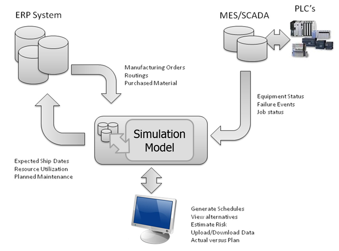
Figure 12.4: Architecture of a typical simulation-based scheduling system.
However there are also some unique challenges in trying to use a general purpose DES product for scheduling, since they have not been specifically designed for that purpose. Some of the issues that might occur include the following:
Scheduling Results: A general purpose DES typically presents summary statistics on key system parameters such as throughput and utilization. Although these are still relevant, the main focus in scheduling applications is on individual jobs (entities) and resources, often presented in the form of a Gantt chart or detailed tracking logs. This level of detail is typically not automatically recorded in a general purpose DES product.
Model Initialization: In design applications of simulation we often start the model empty and idle and then discard the initial portion of the simulation to eliminate bias. In scheduling applications, it is critical that we are able to initialize the model to the current state of the system – including jobs that are in process and at different points in their routing through the system. This is not easily done with most DES products.
Controlling Randomness: Our DES model typically contains random times (e.g. processing times) and events (e.g. machine breakdowns). During generation of a plan, we want to be able to use the expected times, and turn off all random events. However once the plan is generated, we would like to include variation in the model to evaluate the risk with the plan. A typical DES product is not designed to support both modes of operation.
Interfacing to Enterprise Data: The information that is required to drive a planning or scheduling model typically resides in the company’s ERP system or databases. In either case, the information typically involves complex data relations between multiple data tables. Most DES products are not designed to interface to or work with relational data sources.
Updating Status: The planning and scheduling model must continually adjust to changes that take place in the actual system (e.g. machine breakdowns). This requires an interactive interface for entering status changes.
Scheduling User Interface: A typical DES product has a user interface that is designed to support the building and running of design models. In scheduling and planning applications, a specialized user interface is required by the staff that employs an existing model (developed by someone else) to generate plans and evaluate risk across a set of potential operational decisions (e.g. adding overtime or expediting material shipments).
A new approach, Risk-based Planning and Scheduling (RPS), is designed to overcome these shortcomings to fully capitalize on the significant advantages of a simulation approach.
12.8 Risk-based Planning and Scheduling
Risk-based Planning and Scheduling (RPS) is a tool that combines deterministic and stochastic simulation to bring the full power of traditional DES to operational planning and scheduling applications (Sturrock 2012a). The technical background for RPS is more fully described in Deliver On Your Promise – How Simulation-Based Scheduling Will Change Your Business (C. D. Pegden 2017). RPS extends traditional APS to fully account for the variation that is present in nearly every production system, and provides the necessary information to the scheduler to allow the upfront mitigation of risk and uncertainty. RPS makes dual use of the underlying simulation model. The simulation model can be built at any level of detail and can incorporate all of the random variation that is present in the real system.
RPS begins by generating a deterministic schedule by executing the simulation model with randomness disabled (deterministic mode). This is roughly equivalent to the deterministic schedule produced by an APS solution but can account for much greater detail when necessary. However, RPS then uses the same simulation model with randomness enabled (stochastic) to replicate the schedule generation multiple times (employing multiple processers when available), and record statistics on the schedule performance across replications. The recorded performance measures include the likelihood of meeting a target (such as a due date), the expected milestone completion date (typically later than the planned date based on the underlying variation in the system), as well as optimistic and pessimistic completion times (percentile estimates, also based on variation). Contrast Figure 12.3 with the RPS analysis presented in Figure 12.5. Here the risk analysis has identified that even though Order-02 appears to have adequate slack, there is a relatively low likelihood (47%) that it will complete on time after considering the risk associated with that particular order, and the resources and materials it requires. Having an objective measure of risk while still in the plan development phase provides the opportunity to mitigate risk in the most effective way.
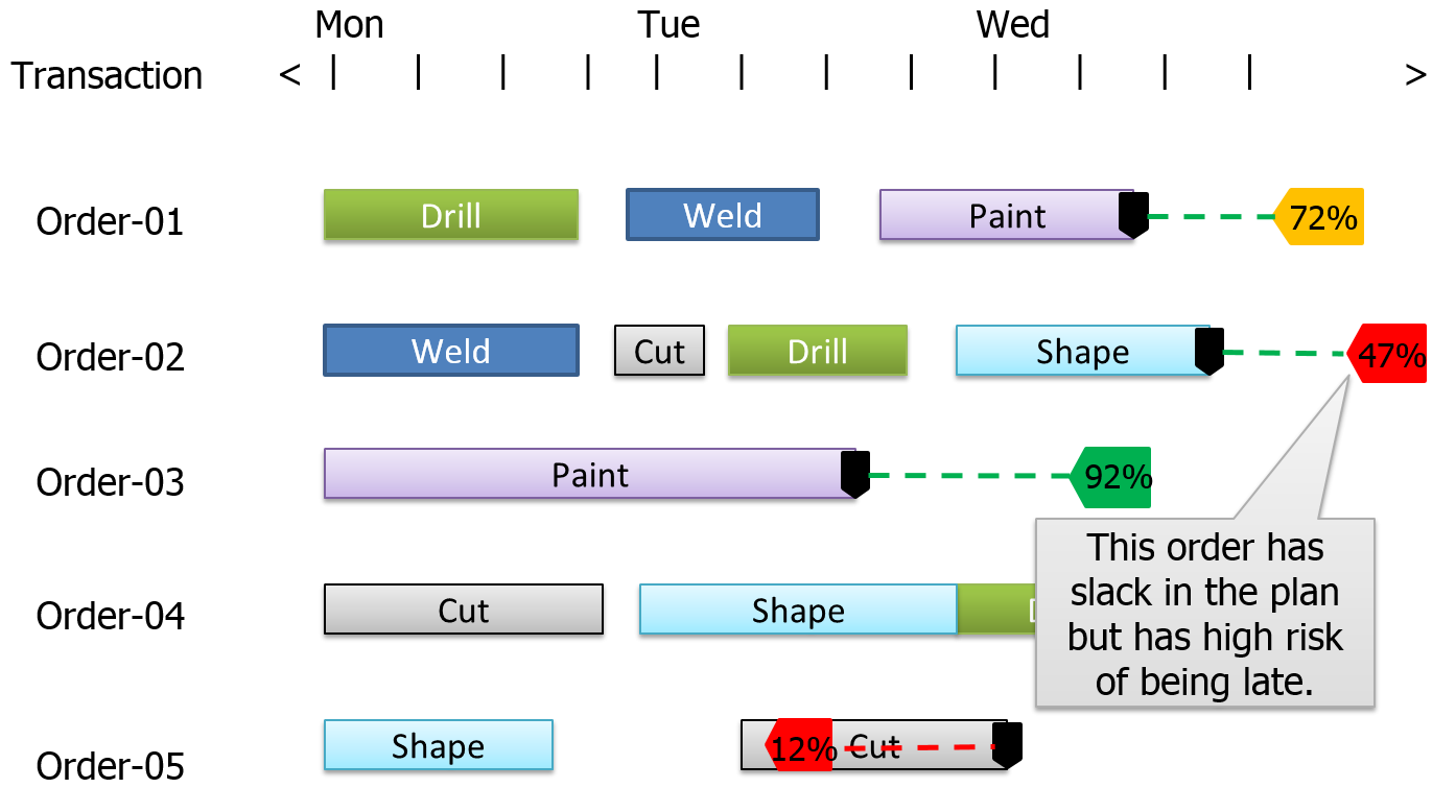
Figure 12.5: Gantt chart identifying a high-risk order.
RPS uses a simulation-based approach to scheduling that is built around a purpose-built simulation model of the system. A key advantage of a simulation-based approach is that the full modeling power of the simulation software is available to fully capture the constraints in your system. You can model your system using the complete simulation toolkit. You can use custom objects for modeling complex systems (if your simulation software provides that capability). You can include moving material devices, such as forklift trucks or AGVs (along with the congestion that occurs on their travel paths), as well as complex material handling devices such as cranes and conveyors. You can also accurately model complex workstations such as ovens and machining centers with tool changers.
RPS imposes no restrictions on the type and number of constraints included in the model. You no longer have to assume away critical constraints in your production system. You can generate both the deterministic plan and associated risk analysis using a model that fully captures the realities of your complex production and supply chain. You can also use the same model that is developed for evaluating changes to your facility design to drive an RPS installation – a single model can be used to drive improvements to your facility design as well as to your day-to-day operations.
RPS implemented as a Digital Twin can be used as a continuous improvement platform to continuously review operational strategies and perform “what-if” analysis while generating the daily schedule. It can be used off-line to test things like the introduction of a new part to be produced or a new machine/line to be installed. “Go-live” of the updated system becomes easy – simply promote the evaluation model to be the live operational model. The model used to prove out the design will immediately affect the schedule based on the system changes without having to re-implement the software or make costly updates or changes.
To ensure better supply chain performance, the model can be extended into the planning horizon to ensure better alignment between the master plan and the detailed factory schedule. The same model will run for 3 to 6 weeks for planning and 1 to 3 weeks for scheduling and perhaps 1 or 2 days for the detailed production schedule for execution. This will then ensure material availability as procurement will be based on the correct requirement dates. This more accurate information can then be used to update the ERP system, for example feeding updates back to SAP.
RPS can even be linked to optimization programs like OptQuest. You can set corporate KPIs and run automatic experiments to find the best configuration for buffer sizes, resource schedules, dispatching rules, etc. to effectively run the factory and then schedule accordingly. Combining the design and execution modes of the simulation model, also makes it an ideal tool for configuring and implementing a Demand Driven MRP (DDMRP) system. A simulation-based DDMRP system has the added advantage of near instantaneous rescheduling and dynamic configuration updates.
12.9 Planning and Scheduling With Simio RPS
Simio RPS Edition is an extended version of Simio that has additional features specifically designed for Risk-based Planning and Scheduling applications. As of Simio Version 16.256 and later this extended capability is now part of every academic package – if you do not currently have it, instructors can apply for an upgrade by sending a request to academic@simio.com. The simplest way to determine whether you have RPS capability is to look for a Planning tab just above the Facility view (Figure 12.6 – many of the RPS features are accessed within the Planning tab). The academic version of Simio RPS is almost identical to the commercial version, but your license prohibits use for commercial applications.
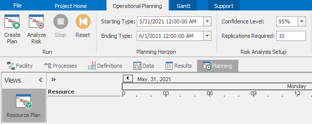
Figure 12.6: The Planning tab provides access to RPS scheduling features.
Although the base model used to drive a Simio RPS solution can be built using any of the Simio family of products, the Simio RPS features are required for preparing the model for RPS deployment. This preparation includes enabling activity logging, adding output states and scheduling targets to tables, and customizing the user interface for the scheduler.
In traditional Simio applications, the data tables are only used to supply inputs to the model. However in RPS applications, the data tables are also used to record values during the running of the model. This is done by adding state columns to table definitions, in addition to the standard property columns. For example, a Date-Time table state might be used to record the ship date for a job, and a Real table state value might be used to record the accumulated cost for the job. Table states can be written to by using state assignments on the objects in the Standard Library, or more flexibly by using the Assign step in any process logic. Output state columns are added to tables using the States ribbon or State button in the Data tab of the Simio RPS Edition.
A scheduling target is a value that corresponds to a desired outcome in the schedule. A classic example of a target is the ship date for a job (we would like to complete the job before its due date). However, targets are not limited to completion dates. Targets can report on anything in the simulation that can be measured (e.g., material arrivals, proficiency, cost, yield, quality, OEE) and at any level (e.g., overall performance, departmental, orders, sub-assemblies, and other milestones).
Targets are defined by an expression that specifies the value of the target, along with upper and lower bounds on that value, and labels for each range relative to these bounds. For example, a target for a due date might label the range above the upper limit as Late, and the range below the upper limit as On Time. Simio will then report statistics using the words Late and On Time. Figure 12.7 illustrates the definition of a target (TargetShipDate) based on comparing the table state ManufacturingOrders.ShipDate to the table property ManufacturingOrders.DueDate. It has three possible outcomes, OnTime, Late, or Incomplete. In a similar fashion, a cost target might have its ranges labeled Cost Overrun and On Budget. Targets can be based on date/time, or general values such as the total production cost. Some targets, such as due date or cost, are values that we want to be below their upper bound; others, such as work completed, are values we want to be above their lower bound. Target columns are added using the Targets ribbon or Targets button in the Data tab of Simio RPS.
Figure 12.7: Defining a target based on table states and properties.
Simio automatically records performance of each target value relative to its defined bounds. In a deterministic plan run, it simply records data on where the target value ended up relative to its defined bounds (On Time, Cost Overrun, etc.). However, when performing risk analysis based on variation and unplanned events, Simio records the performance of each target value across all replications of the model and then uses this information to compute risk measures such as the probability of on time delivery, and the expected/optimistic/pessimistic ship date.
The standard Simio user interface is focused on model building and experimentation. In RPS applications, there is a need for a different user interface that is tailored for the planning and scheduling staff. Schedulers generally do not build models, but instead use models in an operational setting to generate plans and schedules. A separate and dedicated user interface is needed for the planning and scheduling user. Simio RPS lets you easily tailor the user interface for the planning and scheduling staff. You can fully configure the types of data that the scheduler can view and edit, and fully customize the implementation to specific application areas.
12.10 The Scheduling Interface
Up until now, we have been using Simio RPS in Design mode. RPS also has a Scheduler Mode for generating and viewing schedules based on the previously developed model. Scheduler mode provides a customized user interface designed with the planning and scheduling staff in mind. This user interface (Figure 12.8) is smaller and simpler than the standard RPS user interface, since it provides no support for building new models. Scheduler mode executes a Simio model that was built using one of the standard Simio products, and then prepared for deployment using the RPS Design mode. Scheduler mode can be enabled by changing a File \(\rightarrow\) Settings option.
Figure 12.8: Simpler ribbons available in Scheduler mode.
The main purpose of scheduler mode is to generate a plan/schedule by running the planned jobs through the model in a deterministic mode, where all random times are replaced by their expected values, and all random events are suppressed. This deterministic schedule (like all deterministic schedules) is optimistic; however we can then use the features in scheduler mode to analyze random events.
Scheduler mode provides both static and dynamic graphic views of the resulting plan/schedule, along with a number of specialized reports. The graphic views include both entity and resource Gantt charts, as well as a 3D animation of the schedule generations. The entity Gantt chart displays each entity (e.g., a job or order) as a row in the Gantt, and rectangles drawn along a horizontal date-time scale depict the time span that each resource was held by that entity. The resource Gantt chart displays each resource (e.g. machine or worker) as a row in the Gantt, and rectangles drawn along a horizontal time scale depict the entities that used this resource. Both of these Gantt charts are part of the Simio examples that will be discussed later. Figure 12.9 illustrates a resource Gantt chart with the resource constraints partially exploded. It is annotated to identify some contributors to the lateness of Order-04, notably a long time waiting for the weld machine and then additional time waiting for the operator required to run it.
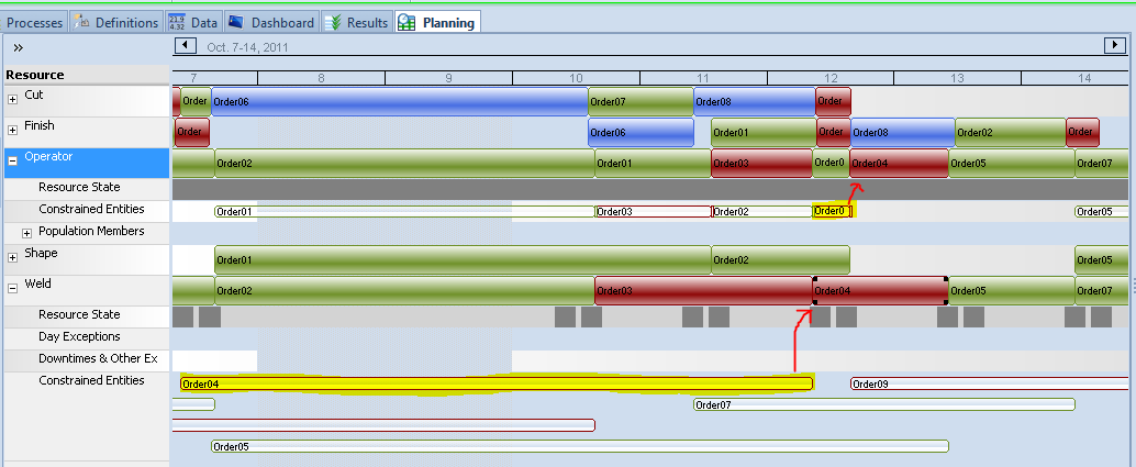
Figure 12.9: Examine constraints to investigate why Order-04 is late.
The specialized reports include a work-to list for each resource. The list defines the start and end time for each operation to be performed by that resource during the planning period. This work-to list is typically provided to the operator of each workstation in the system to provide a preview of the expected workload at that workstation. The specialized reports also include a resource utilization report to show the expected state over time during the planning period, and a constraint report to summarize the constraints (material not available, workers unavailable, etc.) that created non-value added time in the system during the planning period. Figure 12.10 shows an example of a resource dispatch list for an operator. More examples of these reports will be covered in the following examples.
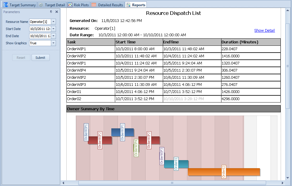
Figure 12.10: Resource dispatch list for operator.
Scheduler mode can also display custom dashboards that have been designed using the design mode to summarize information on a specific job, machine, worker, or material. These dashboards can combine several types of graphical and tabular schedule information into a single summary view of a job or machine to provide additional insights into a plan/schedule.
Scheduler mode allows the planners and schedulers to test alternatives to improve a high risk schedule. Different plans can be evaluated to see the impact of overtime, expediting of materials, or reprioritizing work on meeting specific targets.
12.11 Model 12-1: Model First Approach to Scheduling
In this section we will discuss a model-first approach to building a scheduling model. This approach is most appropriate for new facilities or for facilities where the sub-systems like MES are still under development so model-configuration data is not readily available. While this approach is more time-consuming, since the external data requirements are lower it has the advantage that it can be completed early enough in the process that design improvements identified by the simulation (see Section 12.4) can implemented without major penalties.
We will start by building a simple model, enabling planning features, and reviewing the generated plans. Then we will import a file of pending orders and convert our model to use that data file. We will customize the model a bit more and add tracking of scheduled and target ship dates so we can evaluate the schedule risk. Finally we will briefly explore some of the built-in analysis tools that help us evaluate and use the schedule.
12.11.1 Building a Simple Scheduling Model
Start with a New Project and place a Source, three Servers, and a Sink, then name the servers and connect them with paths as illustrated in Figure 12.11. As you build the model, leave all the object properties at their default values. Group select the three servers and in the Advanced Options property group set Log Resource Usage to True. Set the Ending Type on the Run ribbon to a Run Length of 1 hour.
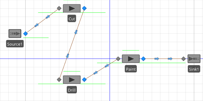
Figure 12.11: Facility window of our simple scheduling Model 12-1.
Select the Planning tab and the Operational Planning Ribbon and click the Create Plan button. When you view the Resource Plan (click top button on the left) you will see each resource listed and on the right side you will see the activity on each resource - more specifically, you will see when each entity started and stopped processing on each resource. If you use the Zoom In or Zoom Range functions on the Gantt ribbon, or simply scroll the mouse on the Gantt time scale, you will be able to more closely examine the activity in a view that looks like Figure 12.12.
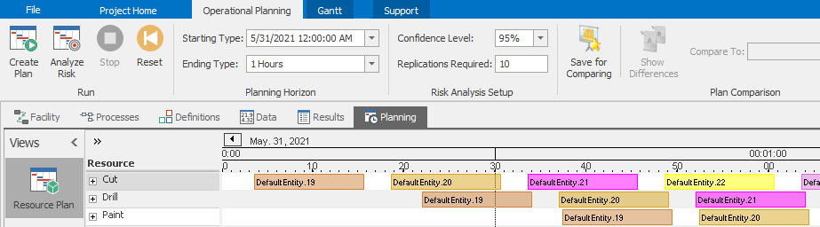
Figure 12.12: Model 12-1 Resource Plan zoomed to show entity details.
If you click the Entity Workflow button on the left, you will see a different Gantt view displaying all entities in separate rows, which resources it used, and when it started and stopped processing on each resource. Again, you can use the Zoom features to zoom in so you can see the detailed activities of the first few entities listed (Figure 12.13). Note that the entity ID’s are sorted as strings (not numerically) - so the first entity created (DefaultEntity.19) comes between DefaultEntity.189 and DefaultEntity.190 – perhaps not intuitive, but we will address that shortly.
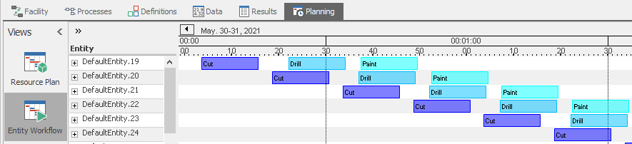
Figure 12.13: Model 12-1 Entity Workflow Gantt zoomed to show resource details.
12.11.2 Making a More Realistic Model
Let’s make our model more realistic by using a data file containing orders we want to produce and using more appropriate processing times. First, back in the Data tab - Tables view we want to go to the Tables ribbon, add a table (Add Data Table button) and name this new table ArrivalTable. You will find a CSV file named ArrivalTableData.csv in the folder named Model_12_01_DataFiles found in the student downloads files. Use the Create Binding button on the Tables ribbon to bind this CSV file to your new table. This action established a relationship between the table and the file, as well as created the schema (column definitions) so we can import the data. With this established, we can now Import the file into the table (Figure 12.14). Since this table has actual calendar dates in it, the model must be configured to run during those dates. On the Run ribbon, set the Starting Type to Specific Starting Time matching the first arrival (12/2/2019 12:00:00 AM) and set the Ending Type to Run Length of 1 Days.
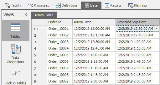
Figure 12.14: Model 12-1 ArrivalsTable after import from CSV file.
In the Facility view select the Source1 object so we can configure it to create entities using the new table. Set Arrival Mode to ArrivalTable and set the Arrival Time property to ArrivalTable.ArrivalTime. Let’s also make the server processing times more realistic. Group select the three servers and change the Units on Processing Time to be Hours instead of Minutes.
The last thing we want to do for now is to use the OrderID listed in the table to identify our entities. Drag a ModelEntity into the Facility view so we can edit its properties. Under the Advanced Options category set the Display Name to ArrivalTable.OrderId. Under the Animation category also set the Dynamic Lable Text to ArrivalTable.OrderId.
We are done with this series of enhancements, so let’s examine our results. Navigate back to the Entity Workflow Gantt under the Planning tab. You should see a bright red bar indicating that we have changed the model since we last ran it, so let’s refresh the Gantt chart by clicking the Create Plan button. After zooming again to adjust to the new times, you should see all your entities listed, now with more meaningful names based on how they were identified in the ArrivalTable (Figure 12.15). And in the Resource Plan, you should see each of your resources as they were, but now the entities again have more meaningful names as well (Figure 12.16).
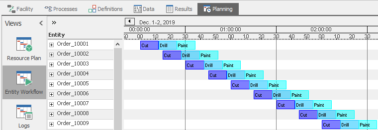
Figure 12.15: Model 12-1 Entity Workflow Gantt with better times and entity labels.
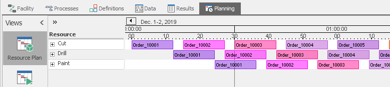
Figure 12.16: Model 12-1 Resource Plan Gantt with better times and entity labels.
12.11.3 Adding Performance Tracking and Targets
Now that our model is working, let’s add a few features to help us evaluate how well our schedule is working. One important item is to record when each order is planned to ship. We do that by first adding a State to our table. Navigate back to the table and select the States. Select a DateTime state to add it to the table. Name this column ScheduledShipDate. This is an output column that is assigned values during the run, so initially it will show errors indicating no data yet. We must assign those values in Sink1, where orders go when they are completed. In the State Assignments section of Sink1 assign ArrivalTable.ScheduledShipDate to TimeNow.
Another important item is to evaluate whether the order is scheduled to be shipped on time. We do that by adding a Target to the table. Navigate back to the Table and open the Targets ribbon. When you click on the Add Targets button, two columns are added to the table - a Value and a Status for that target. Name this target TargetShipDate. The Expression we want to evaluate is ArrivalTable.ScheduledShipDate which has the Data Format of DateTime. The value we want to compare this to is ArrivalTable.ExpectedShipDate - we don’t want to exceed that value so we make it the Upper Bound. You will typically want to replace the default terminology for clarity. Under the Value Classification category set the values of Within Bounds to On Time, Above Upper Bound to Late, and No Value to Incomplete. If you run the model now, you will see that the status of all the orders is Late.
Let’s balance the system by changing the Processing Time for all the servers to be Random.Triangular(0.05, 0.1, 0.2) Hours. Rerun the model and look at our table again. You will see that now almost all of our orders are On Time. If we move over to the Entity Workflow on the Planning tab and run Create Plan, you will see that the plan now has a gray flag on each entity indicating the Target Ship Date. When that flag is to the right of the last operation, that indicates a positive slack time (e.g., the plan calls for that order to complete early). But we don’t yet know how confident we can be in those results. If you click the Analyze Risk button the model will run multiple replications with variability enabled and those flags will change color and display a number that is the likelihood that the order will be On Time.
This model does not yet include much variation, so lets add variation in three places. First, lets allow for variability in order arrival times. If orders typically arrive up to a quarter hour early or up to a half hour late, we would represent that on the Source by setting the Arrival Time Deviation under Other Arrival Stream Options to Random.Triangular(-0.25,0.0,0.5) Hours. Second, let’s assume that the Drill is a bit longer and less predictable than the others and set it’s Processing Time to Random.Exponential(0.2). Finally let’s recognize that all three servers have some reliability problems. Under Reliability add a Calendar Time Based failure to each, leaving the default Uptime Between Failures and Time To Repair. Return again to the Entity Workflow Gantt, click Analyze Risk, and now you will see that even though most orders are still projected to be on time in the deterministic plan, when the variability is considered most of them have a low probability of actually being on-time (Figure 12.17).
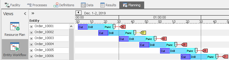
Figure 12.17: Model 12-1 Higher variability system with risk analysis.
12.11.4 Additional Evaluation Tools
All the results and output data that result from the simulation-based scheduling run are available in the Planning tab. It is beyond the scope of this book to describe the analysis tools in detail, but we will mention some of the highlights which we recommend you explore on your own.
On the left panel you will see the tools that are available in Scheduler mode. We have already lightly discussed the two Gantt charts. But there are lots of other Gantt-related features to help you assess and improve the planned schedule. For example if you click on an item in either Gantt, you will see information about the order in the Properties window and if you hover over it you will see a pop-up containing more information about that particular task (Figure 12.18).
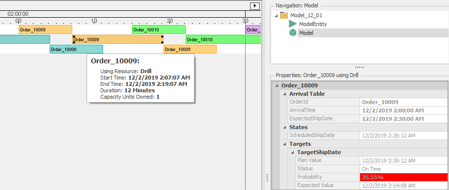
Figure 12.18: Pop-up and properties in a Gantt.
Although our example model so far doesn’t require it, clicking the + button to the left side of a row displays more detail about the items in that row (like Constraints). The buttons on the Gantt ribbon control which optional data can be displayed. Both of these are illustrated in Figure 12.19.
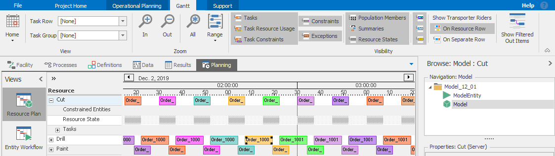
Figure 12.19: Displaying additional row data in a Gantt.
The third button on the left displays Logs which record and display all of the events in ten categories including resource-related, constraints, transporters, materials, and statistics. The Gantt charts and many of the other analysis features discussed below are built on the data in these logs. You can filter these logs to make them easier to read. You can also add columns to the logs to better identify your data.
The Tables button on the left produces a tabbed display similar to the tables we have already used under the model’s Data tab. The key difference is that the model builder can choose which columns in each table appear (versus hidden from the scheduler) and which columns may be changed by the scheduler (versus display only). You can use this to simplify the table and protect the system from changes that the scheduler is not allowed to make (e.g., changing a expected ship date). If you run a risk analysis, the Planning view tables will have extra columns added displaying the results of that analysis.
The Results button at the very bottom on the left enables a third row of tabs (like we didn’t already have enough tabs!) The Target Summary illustrated in Figure 12.20 along with the Target Detail, and Risk Plots provide successively more detailed risk analysis data. The Detailed Results tab shows a pivot table that is very similar to what is available in the interactive run. The Reports, Dashboard Reports, and Table Reports provide the ability to view predefined or custom reports, or even interactive dashboards, tailored to the needs of the scheduler and other stakeholders.
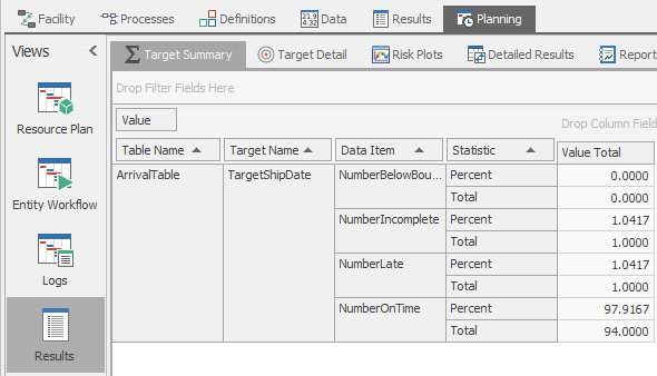
Figure 12.20: Displaying target summary data.
Collectively, these tools allow schedulers to understand why their plan is performing the way it is, help analyze potential improvements, and allow sharing results with others.
12.12 Model 12-2: Data First Approach to Scheduling
In Section 12.11 we practiced building a partially data-driven model with the model first approach. In Section 7.8 we discussed some of the theory and practice behind data-generated models. This latter approach is appropriate when you have an existing system and the model configuration data already exists in ERP (e.g., SAP), MES (e.g., Wonderware), spreadsheets, or elsewhere. A significant benefit of this approach is that you can create a base working model much faster. Now that we have a bit more modeling and scheduling background, let’s build a model from B2MML data files (Section 7.8) and then explore how we might enhance that model. The system we are modeling has two machines to choose from for each of four operations as illustrated in Figure 12.21.
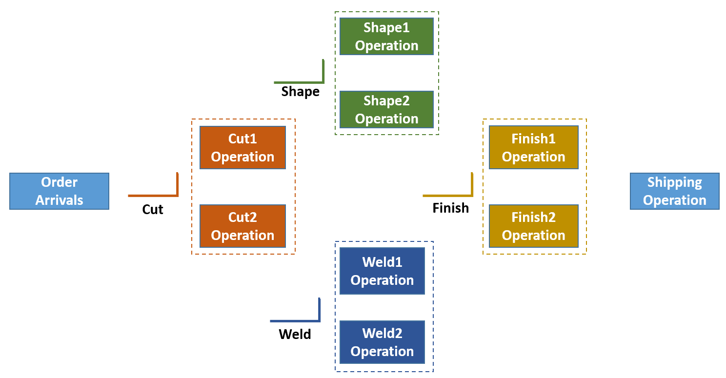
Figure 12.21: Model 12-02 system overview.
Each product will have its own routing through the machines. We will start by using some built-in tools to setup the data tables and configure the model with predefined objects that will be used by the imported data. Then we will import a set of B2MML data files to populate our tables. We will also import some dashboard reports and table reports to help us analyze the data.
12.12.1 Configuring the Model for Data Import
Simio B2MML compliant tables include: Resources, Routing Destinations, Materials, Material Lots, Manufacturing Orders, Routings, Bill Of Materials, Work In Process, and Manufacturing Orders Output. We will be creating all of these tables and importing all except the last one. But before we can import them, we will configure the model for their use. To do this we press the File button then press New From Template. This will bring up a set of templates as illustrated in Figure 12.22.
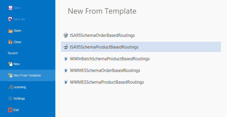
Figure 12.22: Scheduling buttons to prepare for B2MML data input.
The ISA95SchemaProductBasedRoutings template generates B2MML compliant tables, so we will select this template for this model. After selecting the ISA95SchemaProductBasedRoutings template, the Resources, Routing Destinations, Materials, Material Lots, Manufacturing Orders, Routings, Bill Of Materials, Work In Process, and Manufacturing Orders Output tables can be seen in the Data tab.
12.12.2 Data Import
We are now ready to import the data. Select the Resources table. Choose the Create Binding option, select CSV, and select the file named Resources.csv from the folder named Model_12_02_DataFiles found in the student downloads files. Then click the Import button on the Table ribbon. If you navigate to the Facility view, you will see that the resources have been added to the model.
Navigate back to the Data tab. Repeat the above process with each of the seven other tables, binding each to its associated CSV file, then importing it. If you navigate back to the Facility view, you will see our completed model. The navigation view of Figure 12.23 illustrates the objects that were added to this model when you clicked the Import button. If you select the Shape1 object, you can see in the Properties window that it is a SchedServer object and that many of the properties like the Work Schedule, Processing Tasks, and Assignments have been preconfigured to draw data directly from the tables.
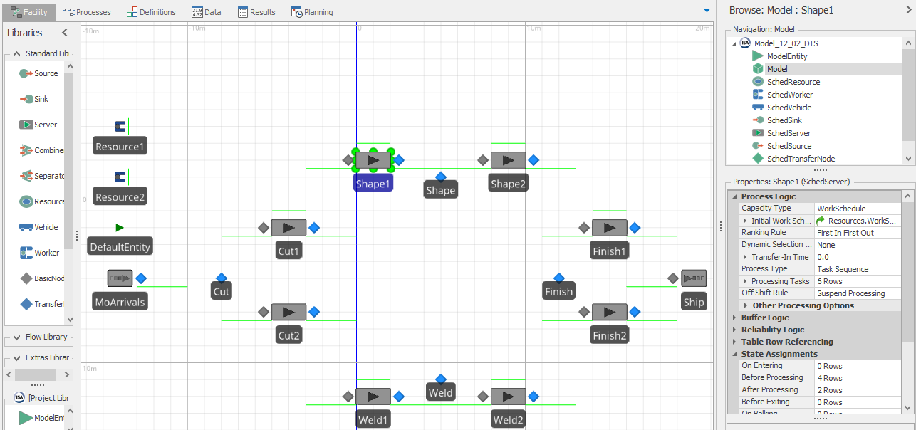
Figure 12.23: Model 12-02 after data import is completed.
12.12.3 Running and Analyzing the Model
Our model has been completely built and configured using the data files! You can now run the model interactively and see the animation. Before we run, there is an important detail that requires our attention. The example data we just imported includes order Release Dates and Due Dates from December 2017 – if you execute the model at the current date, all your orders will be quite late. The easiest thing to do is to change the model starting type (starting time) to 12/2/2017 8:00.
Before we can use this model for scheduling we must go to the Run ribbon Advanced Options and select Enable Interactive Logging. Note that each custom object we used already has its option set to log its own resource usage. Now you can go to the Planning tab and click the Create Plan button to generate the Gantt charts and other analysis previously discussed.
Let’s import some predefined dashboards that were designed to work with this data schema. These dashboards are saved as XML files and can be found in the same folder as the CSV files. The three dashboards provide material details, order details, and a dispatch list for use by operators. To import these dashboards, go to the Dashboard Reports window of the Results tab (not the Results window under Planning) and select the Dashboards ribbon. Select the Import button and select the Dispatch List.xml file from the same folder used above. Repeat this process with the Materials.xml file and the Order Details.xml file. If you go back to the Planning tab \(\rightarrow\) Results window \(\rightarrow\) Dashboard Reports sub-tab, you can now select any of the three reports for display. Figure 12.24 illustrates the Order Details dashboard report.
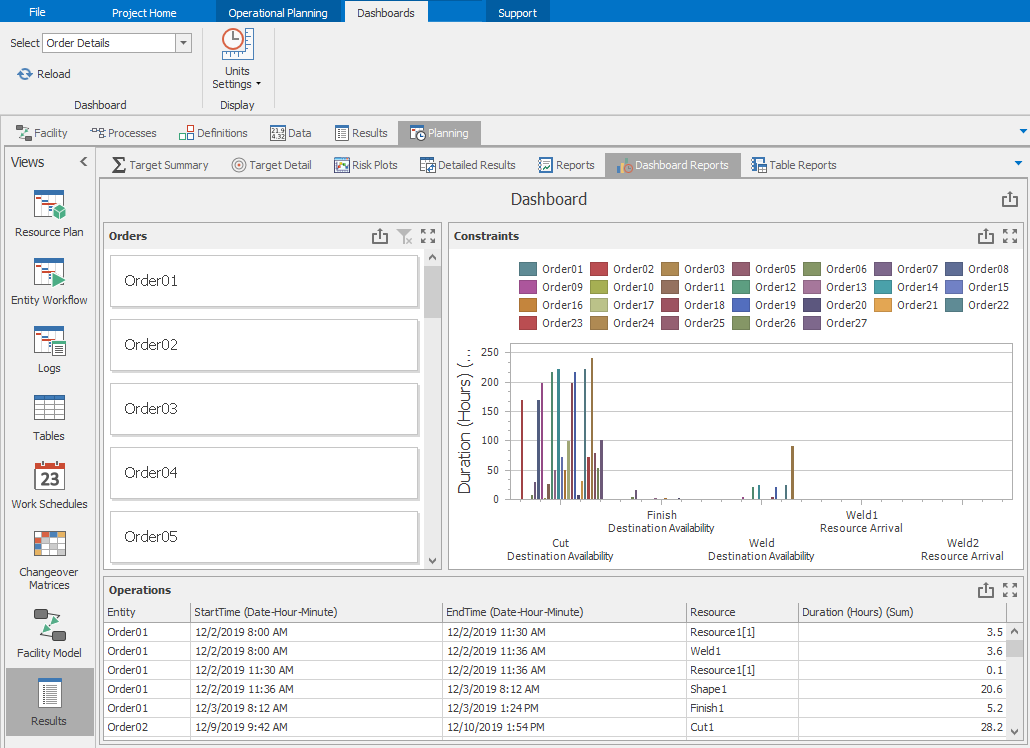
Figure 12.24: Order details dashboard report for Model 12-02.
Finally, lets add a couple traditional reports. To import these reports, go to the Table Reports window of the Results tab (again, not the Results window under Planning) and select the Table Reports ribbon. Select the Import button for ManufacturingOrdersOutput and select the Dispatch List Report.repx file from the same folder used above. Repeat this process Importing for ManufacturingOrders with the OrderDetails.repx file. Importing these two files has now defined the reports for use in the Planning tab. If you go back to the Planning tab \(\rightarrow\) Results window \(\rightarrow\) Table Reports sub-tab, you can now select either of the two new custom reports for display.
While this was obviously a small example, it illustrates the potential for building entire models from existing data sources such as B2MML, Wonderware MES, and SAP ERP systems. This approach can provide an initial functioning model with relatively low effort. Then the model can be enhanced with extra detail and logic to provide better solutions. This is a very powerful approach!
12.13 Uniko Scheduling Case Study
Uniko Designs Grupo (Uniko) is a small Guatemalan company founded in 1999 dedicated to the creation of unique spaces to share with family members, manufacturing architectural finishes, wooden furniture (kitchen & other spaces), Melamine and MDF board furniture for interior and exterior. They employ a team of professionals to develop proposals, build, and install the requested enhancements. They are in a market with growing local and regional demand for kitchens, closets, and pergolas . The company is expanding and modernizing.
The increased product volume, new employees, and new manufacturing techniques have stressed their existing infrastructure. As a small company most people had multiple skills making it hard to determine the best staff assignments. They used a simple spreadsheet-based system to estimate order completion dates (capable to promise) and to make day to day management decisions in staffing and prioritization. The introduction of new equipment and software provided opportunities to improve their production but with so many concurrent changes it was hard to visualize how to maximize their production by using the most efficient assignment of resources.
They requested a tool to replace their existing spreadsheet that would include their machines, workers, processes and alternate processing options. This tool must be able to:
- Aid understanding of the process details and interactions.
- Allow them to test alternate staffing and production sequences to determine the best way to meet their production demands.
- Generate daily work schedules. It should automatically prioritize customer orders and reallocate resources to provide the best overall results and ensure that the most important orders are delivered on time.
- Determine capable to promise (CTP), with accurate schedules representing all current orders through delivery and installation. When a new order is proposed the tool should provide a good estimate of when the new order can be completed.
- Even given all the above, they wanted to leverage their familiarity with Excel and use that as data input to the tool.
It was determined that a fairly simple data-driven Simio model could meet Uniko needs. Because they were unfamiliar with simulation technology, the model was built in small phases giving them the opportunity to try each phase. This provided the opportunity to learn the technology, determine and prioritize their most important needs, and keep the model and data interface as simple as possible. After they tested each phase, they then requested additional enhancements to improve the tool results and usefulness.
12.13.1 Model 12-3: Base Uniko Model
In this section we will build the base Uniko model together. Then you will explore some requested enhancements in the homework problems. As we build, one of our goals is to keep the model and its data files as simple as possible to ease learning and use of the model. So we will start with the Agile modeling premise that we will implement the simplest thing that will meet our immediate objectives, then evaluate the performance and enhance the model as needed.
Here is a high-level overview of what we know at the start of the project:
Uniko has four main products that they produce: Small Kitchen, Medium Kitchen, Large Kitchen, and Pergola (see Figure 12.25). While they have many variations of each of these and some other minor products, these four products account for most of the business. We will add these four products to the model as entity types.
Work is performed at 16 locations (Servers) plus the entry (Source) and exit (Sink). All of the locations have a lot in common. At this point we don’t know of any customization required, but it is often wise to start with a custom object definition. So we will create a custom server object that is subclassed from the Standard Library Server.
Work is performed at locations by 20 different job classes (Resources) each with a specified capacity (number of people). Since these are likely to change as the workforce changes this will be represented in a “Resources” data table which is populated from a spreadsheet. The resources might also require customization later so we will create a custom resource object that is subclassed from the Standard Library Resource.
While each of their four products are processed at the same shared locations and by the same shared resources, they have different process times and resource requirements, and some products skip some locations. Since this is also expected to change as they refine their processes, this will be represented in a “Routings” sequence table that can be imported from a spreadsheet.
And finally we need an “Orders” table to represent the customer orders and important descriptive information (like due dates). This will be changed very often and so will also be imported from a spreadsheet.

Figure 12.25: Uniko products including sample kitchens and a pergola.
While many scheduling models start with the use of a template, we will not do that because our data needs as specified above are relatively simple. In this simple model we do not need the overhead of the extra data tables and custom objects. So let’s get started with the base model:
- Create a new model named
UnikoBaseModel.spfx. We want this to be a data-generated model so the users can interact mostly via spreadsheets. You might want to review Sections 7.7 and 7.8 before proceeding. - On the Table window, add a data table named
JobTypes. - Add two Real properties named
XLocandZLocrespectively. - Add an Object Reference Type column of type
Entity. Name itJobType. - Change the Default Value Instantiation property to
AutoCreateInstance, so that we can automatically populate entity types from an external file. - Change the Object Type property to
ModelEntity. - Open the Initial Physical Characteristics property and define the X property as
XLocand the Z property asZLoc. This will define the X/Z coordinates where the entity will be instantiated. While we are there, let’s change the Length and Width each to1, so they will be a little bigger to see in the model. - Since this is a small table, let’s go ahead and populate the four entity types as illustrated in Figure 12.26. If you look over to the Facility window, you should now see the four entity types to the upper left of the 0,0 center point.
- Assuming that everything works, go back to the Data window, select the Content tab, and select
Save to CSV. Look at the generated file (often a CSV file will automatically load into Excel or another spreadsheet program). It should look similar to the Simio table. Close the CSV file. - Now lets set up a data connector so we can import into this table. Still on the Content tab, select
Create Bindingand then CSV Data Importer from the pull down list. Name itCSV Data Importer JobType. Go to the Data Connectors button on the left and add the filenameJobTypes.CSV. If you hit the ‘+’ key you should see the file contents as illustrated in Figure 12.27. - Back on the Content tab, you can press the
Import Tablebutton to import that file. The contents should not change unless you manually changed something, but the table heading should change to indicate that the import just happened.

Figure 12.26: Model 12-03 initial jobTypes table.

Figure 12.27: Uniko jobTypes table data connector.
Let’s move on to our Resources (in this case our workers). We will take a different approach here and build the table from an existing data file.
- As mentioned above, it seems likely that we might want to customize the resources, so let’s add a custom Resource. In the Facility window, right click on the Resource in the Library and select
Subclass. You should now see a new object named MyResource in the upper right Browse window. This is presently an exact copy of the Resource, but it can now be edited as needed. Right click on MyResource and Rename it toUnikoWorker. - We do not want to continue editing the UnikoWorker now, so navigate back to the (main) Model. Then return to the Data and Tables window on our main model.
- Add a Table named
Resources. - From the Content tab Create Binding of type CSV Data Importer, and name it
CSV Data Importer Resources. - On the Data Connectors page, add the filename
Resources.CSV(a supplied file). - Back on the Table window, Content tab, you can now “Import Table”. The data should now be there, but we still need to add some options since by default everything came in as strings and numbers.
- In the Schema tab, click on the Capacity column and select Change Type, then select
Standard Property and Integer. - Click on the Resource Name column and select Change Type, then select
Object Reference and Object. - Select Object Type of our new
UnikoWorker.
- Change the Default Value Instantiation property to
AutoCreateInstance. - Open the Initial Physical Characteristics property and define the X property as
XLocand the Z property asZLoc. - Change Auto-set Table Row Reference to
True.
If you visit the Facilities window, you will now see all of the Workers (resources) populated.
The next section we will add the Locations (often machines) where the work is done. For these we will create a customized Server object to make it easy to make changes to the location behavior.
- In the Facility window, right click on the Server in the Library and select Subclass. Right click on MyServer and Rename it to
UnikoLocation. - Back in the main model create a table named
Locationsand follow a similar procedure above to connect it to the supplied fileLocations.csv, import the data, change the column types and configure the table. - If you were successful, you should see all 16 locations in the Facility window.
- To complete the process flow we need to add two additional objects, a Source and a Sink. Add a Source named
OrderEntryat approximately coordinates -10, -30 (to the left of the first location). Leave the properties at their defaults for now. Add a Sink named17OrderCompleteat approximately coordinates 50, 40 (to the right of the final location).
Most of our model is now complete. The Facility window should now look like Figure 12.28. Note that all the objects we have defined are there, but no connectors are used. We will drive entities through the system based on Routings that are defined and imported in a Sequences table.

Figure 12.28: Model 12-03 facility window.
The next table to import will be the Routings (sequences) table to describe how each product will be produced. At each step a product will have a specified team of resources - varying quantities of up to three different resource types. And that team will require a product-specific time to process.
Create a table named
Routingsand follow a similar procedure above to connect it to the supplied fileRoutings.csvand import the data.Change the column types as specified here:
- JobType will become a foreign key, relating to the JobTypes table. So first we must go to the JobTypes table, select the JobType column, and select the
Set Column as Keybutton. Success will be indicated by a key icon in the JobType column header. This will be the single location that defines products, all other locations will reference back to this table. Now we can go back to the JobType column in the Routings table and Change Type toForeign Key. Success here will be indicated by a key icon in each field in that column. You must also tell it which key to use by setting Table Key toJobType.JobTypes. - JobStep should be defined as an Integer. This is here simply to make it easier to move around in the sequence.
- Location should be defined as a Standard Property > Sequence Destination. This will be the primary way that entities will move through the system. Set the Accepts Any Node property to
False, since for ease of use we are using a server name instead of an input node. - ProcessTime is a Real property, but it should be specified with a Unit Type of
Timeand Default Units ofHoursand also have its Required Value set toFalse. - The last 6 columns are actually 3 pairs of columns. While most locations require a single resource class, some require more than one unit of a resources, and some require 2 or even 3 resources (or even no resources at all).
- Resource1 is the primary resource needed at that location. It should be specified as an Object Reference > Object property. The Filter to Resources property should be set to
True. The Required Value should be set toFalse, since some locations may require no resources. - Quantity1 is the quantity of Resource1 needed (if any). It should default to 0 and also have its Required Value set to
False. - Make similar changes for Resource2, Quantity2, Resource3, and Quantity3.
- Resource1 is the primary resource needed at that location. It should be specified as an Object Reference > Object property. The Filter to Resources property should be set to
- JobType will become a foreign key, relating to the JobTypes table. So first we must go to the JobTypes table, select the JobType column, and select the
Our final table will be an Orders table to specify what will be produced. While the ultimate customer will want this file in an external file, we will start by making it just a data table so we can enhance it as needed.
- Create a new data table named
Orders. - Add the following columns:
OrderID, an integer.JobType, a Foreign Key Property, using the Table Key JobTypes.JobTypePriority, an integer.ReleaseDate, a real property (for now) that has UnitType ofTimeand Units ofHours.
- For testing purposes, lets add two orders, #1 a
SmallKitchenand #2 aLargeKitchenleaving the other properties at their defaults of 0.
Let’s use the Show Table Schema Viewer on the Schema tab to look at the overview of our present table schema (see Figure 12.29). You can see graphically how the Routings table and the Orders table reference the JobType key in the JobTypes table.
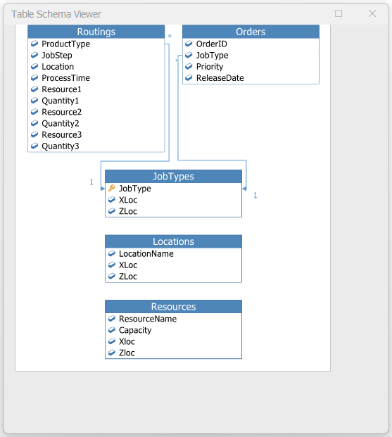
Figure 12.29: Model 12-03 initial table schema.
Although all our data is done (for now) we still have to modify the model to use all that data. Lets start by getting our orders into the model.
Edit the OrderEntry Source object to use:
- Entity Type of
JobTypes.JobType - Arrival Mode of
Arrival Table - Arrival Time Property of
Orders.ReleaseDate - Entity Destination Type on the exit node to
By Sequence
- Entity Type of
Lets update the first location (01Blueprint) to use the data in the tables:
Change Ranking Rule to
Smallest Value Firstusing Ranking ExpressionOrders.Priority.Change Processing Time to
Routings.ProcessTime.In the Secondary Resources category, open the repeat group for Resources For Processing. In here we will add one repeat line for each processing tuple:
- Resource Name
Routings.Resource1, Units Per ResourceRoutings.Quantity1 - Resource Name
Routings.Resource2, Units Per ResourceRoutings.Quantity2 - Resource Name
Routings.Resource3, Units Per ResourceRoutings.Quantity3 - But wait, you may think, some of these fields are not used. That’s OK because Simio Seize has a useful feature that if the resource name is blank or the quantity is 0, that line is just ignored. When complete it should resemble Figure 12.30.
- Resource Name
In the Advanced Options Category change the Log Resource Usage property to
Trueso that we can see this item in the Gantt chart.Change the Entity Destination Type on the exit node to
By Sequence.
At this point you may be anticipating making similar changes on the other 15 locations. But I have good news! Because all these locations were based on the same custom object (UnikoLocation), there is a much easier way. Right click on the 01BluePrint object we have been changing and select the option Update 'UnikoLocation' Property Defaults from This. As the name might imply, all the changes we made to the 01Bluprint object instance have been copied into the UnikoLocation object definition. Now all 16 location object instances will link to the data tables in the same way!

Figure 12.30: Model 12-03 resources specified from Routings table.
We need to make an update to the UnikoWorker as well. We will do it in the same way. Edit the SalesAgent instance to set Initial Capacity to Resources.Capacity. Right click on the SalesAgent object we have been changing and select the option Update 'UnikoWorker' Property Defaults from This. Now all 20 worker object instances will get their capacity values from the data tables.
We should now be ready to run and watch the Facility window. Since the Routings calls for each operation to take from 4 to 40 hours, it will appear to run very slow. I suggest setting the Speed Factor on the Run ribbon to something like 1000. If you run you should see the two orders start to sequentially move down the first column of locations for the default specified 24 hours of run time.
On the Run ribbon, let’s set the Ending Type to Unspecified (Infinite). Recall this allows the model to run until in runs out of events – in this case that means it will complete all the orders and then stop. Open the Planning window and push the Create Plan button on the Operational Planning tab. Recall that pressing the All button on the Gantt tab will automatically scale the Gantt windows to show all orders through their completion (or model end, whichever comes first). In the Resource Plan window you should see a line for each location and an indication of what entity was using it over time (see Figure 12.31). In the upper half of the window you will notice a flow where the first order started proceeds unimpeded through all the locations, but the second order is initially constrained waiting for the first order. In the lower half of that same window you can see each worker and what they are working on over time.

Figure 12.31: Model 12-03 resource gantt with two orders.
If you switch to the Entity Workflow window you should see a line for each entity (order) and an indication of what resources that entity was using over time (see Figure 12.32). If you expand the constraints by selecting the +, you can clearly see that the start of the second order was delayed waiting for availability of the 01Blueprint location, and then later slightly constrained by the 03FinalBluprint location. In this case you don’t see additional constraints because the second order (LargeKitchen) process times on each step are generally longer. If the orders had been released in reverse order, you would have seen more significant conflicts.

Figure 12.32: Model 12-03 entity workflow gantt with two orders.
12.13.2 Model 12-4: Uniko Model Enhancements
You will recall previously that the customer wanted a model that was easy to use – that also implies having the simplest model that might possibly meet their needs. Now that we have a complete but still very simple model that we can play with a bit, we can incrementally add more features as they identify additional needs. In this section we will address some of those additional requirements.
Before we add more features, we should do some additional testing to help validate the model. It is often easier to do such validation before we add more complicationg features. A bare minimum test might be to run four orders, one of each job type, through the system. Then we can examine the animation, trace, and Gantt displays to convince ourselves that the model is working as designed. If you have added one order of each type, in the order they were defined, you should see a Resource Plan that the upper half looks something like Figure 12.33 and an Entity Workflow that looks something like Figure 12.34.

Figure 12.33: Model 12-04 resource gantt with four orders.

Figure 12.34: Model 12-04 entity workflow gantt with four orders.
Now that we have a bit more work in the system, it looks more realistic – except that it looks a little too busy. One of the first additional requirements the customer identified was that their entire staff followed a schedule where they worked five full days and a half day on Saturday. The locations are always available, but the workers all follow the same single shift per day. So lets add a schedule to make that happen:
- If you navigate to the Data > Work Schedules window, you will see that Simio has already defined a Work Schedule named StandardWeek, that is a 7 day week consisting of four 8-hour StandardDays. This is pretty close to what we need, so we will just build on that.
- The StandardDay is defined as two four-hour work periods with a mid-day break. This suites the customer. But we must reflect here that the capacity (Value property) must get its data from the Resources Table. So change both Value properties to
Resources.Capacity. - We also need to add a new Day Pattern for the half-day on Saturday. Create a new Day Pattern named
HalfDaythat looks just like the morning part of the StandardDay. - Now go back up the the StandardWeek definition and add a
HalfDayon Saturday. When you have completed these steps, it should look like Figure 12.35. - Now that we have created the schedule, we must tell the UnikoWorkers to follow it.
- Select SalesAgent (or any UnikoWorker) and in the Properties window change Capacity Type to
WorkScheduleand verify that Initial Work Schedule isStandardWeek. - Right click on the object and select the option
Update 'UnikoWorker' Property Defaults from This. Now all 20 worker object instances will follow the specified schedule, each at their own capacity as specified in the table.
- Select SalesAgent (or any UnikoWorker) and in the Properties window change Capacity Type to
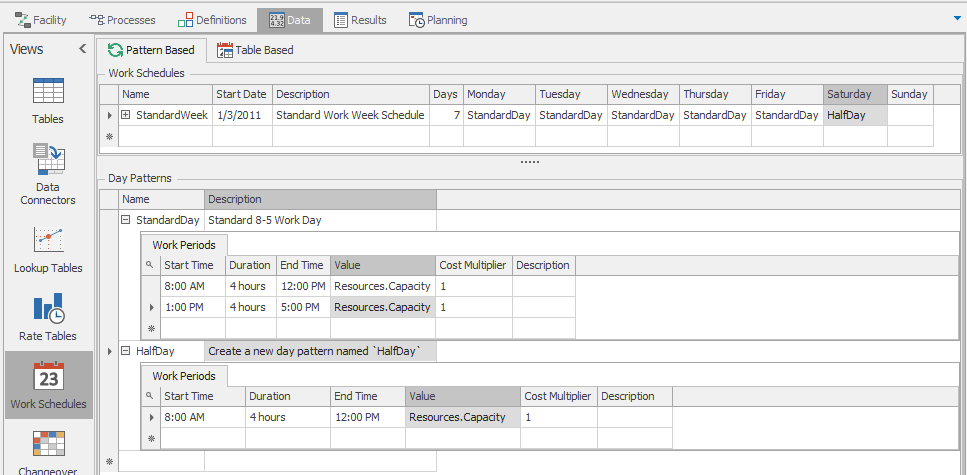
Figure 12.35: Model 12-04 schedule defined to work five and one half days per week.
If we run the model and look at the Resource Plan again (Figure 12.36) it looks superficially the same. But while the entire schedule of four orders was previously completed in about 14 days, it now requires about 55 days. Why? Because the resources are now available only 44 hours per week instead of 168 hours per week.

Figure 12.36: Model 12-04 resource gantt with four orders following a schedule.
The next set of customer enhancements requested are related to better definition of the orders. They want a customer name (a string) associated with each order. And they want the OrderID combined with that string to be used to identify orders in the model.
- Change the type of OrderID to
String. - Add a column of type String, named
Customer, and move it to the second column.
They also want to work with actual dates instead of integers and to not only have a Release Date, but also a Promised Date. On the Orders table, make the following changes:
- Change type of Release Date to Standard Property
DateTime. Change the default to01/01/2025. - Change all the release dates to
1/1/2025. - Add a new Property of type
DateTimeand name itPromisedDate. Change the default to01/01/2025. - Since they anticipate a standard processing lead time of 6 weeks, change all the promised dates to
2/15/2025. - On the Run ribbon we will change the Starting Type to
1/1/2025 12:00:00 AM.
To implement both of the above changes into the model, edit the SmallKitchen object instance:
- Under the Advanced Options category change Due Date Expression to
Orders.PromisedDate. - Under the Advanced Options category change Display Name Expression to
Orders.OrderID + ":" + Orders.Customer. - Under the Animation category change the Dynamic Label Text to
Orders.OrderID + ":" + Orders.Customer. - Right click on the object and select
Update 'ModelEntity' Property Defaults from This. Note that not all properties are always updated with this technique. For example you may need to right click on the Dynamic Label text in each entity object instance and clickResetto get it to use the new default value.
This would be a good time to run the model interactively, generate a plan, and verify that the changes we just made are working correctly. For example, with some extra sample data added the Orders file looks like Figure 12.37
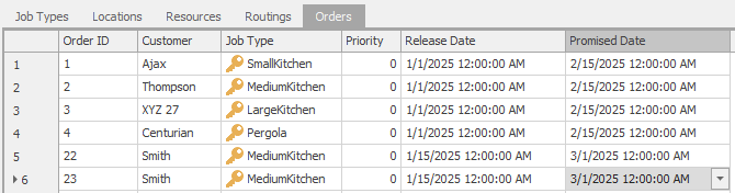
Figure 12.37: Model 12-04 sample orders for testing.
You can see the new labeling in Figure 12.38 as well as the two new orders that were to be released January 15.

Figure 12.38: Model 12-04 Resource Plan with new order ID and later order releases.
The final set of customer enhancements that we will cover here is the implementation of basic WIP. They would like to be able to generate a plan on say February 1 that includes orders that have been started earlier, say in January. They do not have detailed progress on each order, but they do know which job steps have been completed on each order. This will require a couple changes to the Orders table as well as minor changes to the model.
- Add a new column of type Integer named
LastCompletedStep. Move this column just to the right of JobType. The customer can complete this with the last step number that has been completed. For example if step 7 has been completed on an order, this field would be set to 7. - Add a new column of type Expression Property named
CalcReleaseDate. It should have a Unit Type ofTimeand Default Units ofHours. The default Value should be the expressionMath.Max(TimeNow,Orders.ReleaseDate). The value of this column will always be calculated based on the current time so that any orders released in the “past” (e.g., before the model starts running) will instead be released at the time the model starts. This will be combined with the LastCompletedStep to represent WIP.
We need to make a few changes to the OrderEntry (Create) object in the Facility view:
- Under Entity Arrival Logic change Arrival Time Property to use
CalcReleaseDateas explained above. - Under Add-On Process Triggers > Created Entity create a process containing a SetRow step. Specify the Table Name as
Routingsand specify the Row Number asOrders.LastCompletedStep. This will override the default association to make each order start at just after the specified job step. If the value is 0, it will start normally at step 1. If the value is anything else, it will start at next specified step in the routing. - Finally under State Assignments > Before Exiting add an assignment to the State Variable Name
ModelEntity.Priorityof the New ValueOrders.Priority. This is unrelated to the previous changes, but sometimes it is convenient to have such basic information as entity priority readily available in the existing entity state. The customer has requested that lower priority values be considered more important than higher values, so we have recommended that a “standard” priority be set to 10 or above, leaving lower numbers available to expedite priority orders.
The enhanced Orders file looks like Figure 12.39.

Figure 12.39: Model 12-04 enhanced orders for testing.
Again, this would be a good time for you to try various scenarios in the Orders file to ensure that orders are starting processing just after the specified step. And try changing the Starting Type (date) to some time after some orders have already been started to ensure that WIP is represented correctly.
12.13.3 Uniko Model Results
Use of the base model plus enhancements (including some not covered here) helped Uniko maintain and increase production as new equipment was installed. Rather than just guessing how the new process would flow, the model provides an objective look ahead helping them anticipate potential problems before they occur. They can also exercise “what if” scenarios to discover new and unanticipated ways to do things.
They use this model on a regular basis to help manage work assignments and order priorities. When orders do not proceed as planned (perhaps material arrives late or a key person calls off), the model can help them evaluate alternative actions. They can estimate delivery dates with high confidence and learn about any developing problems early enough that they can be resolved without resulting in a late delivery or an unhappy customer.
The tool also provides assistance in accepting and pricing new work. If a potential customer requests an aggressive delivery date, Uniko can use the model as a “Capable to Promise” tool to evaluate if the order date is possible, what extra resources (e.g., overtime) might be required, and what trade-offs (e.g., putting other customer orders at risk) might be involved.
12.14 Additional Information and Examples
12.14.1 Simio E-books on Planning and Scheduling
The Simio website includes the e-book Manufacturing Digital Twin, Solution Description. You can find this on the Textbook Publications page (https://textbook.simio.com/) or via the Books button on the Support ribbon. This is an excellent place to continue your exploration of simulation-based scheduling. This book covers the standard data schemas and many of the general scheduling concepts and how each of those is addressed in Simio.
At the same location you can also find the e-book Deliver on Your Promise: How Simulation-Based Scheduling will Change Your Business. This book is great for managers who want a better understanding of the complex process of scheduling. This provides more details on some of the topics discussed in this chapter as well as describes a few case studies. You are encouraged to share this pdf (or the printed version available on-line) with managers who are looking to solve their scheduling problems.
12.14.2 Scheduling Examples
The Simio software includes six scheduling example files that are each also documented in accompanying pdf files. These files are located under the Examples button on the Support ribbon.
12.14.2.1 Scheduling Discrete Part Production
The system to be scheduled in this example is a discrete part manufacturing facility. The facility is a job shop that produces three finished goods, each with its own routing and unique setup, processing time, and material requirements, at each machine within its routing. We wish to generate a 30-day production schedule that fully accounts for the limited system resources. The facility consists of functionally grouped machines with parts that are dynamically routed based on scheduling rules. Some machines require a secondary resource and/or have sequence dependent setup times. The B2MML-based data schema discussed in the scheduling overview document is used to hold the production data for this example.
12.14.2.2 Scheduling Bicycle Assembly
The system to be scheduled in this example is a bicycle assembly facility. The facility is a job shop that produces finished goods on a final assembly line as well as parts or components for final assembly based on the customer orders. The schedule also includes a number of purchased parts required for final assembly. We wish to generate a seven day production schedule for this facility that fully accounts for the limited resources and parts in the system.
12.14.2.3 Scheduling Bicycle Assembly - Update MO and POs
This is an expansion of the above Scheduling Bicycle Assembly example. It also determines, from sales orders, the manufacturing orders and purchase orders that should be generated based on initial inventory in the system. We wish to generate a 14-day production schedule for this facility that fully accounts for the limited resources and parts in the system.
12.14.2.4 Scheduling Batch Beverage Production
In this example, we generate a 30-day production schedule that fully accounts for the limited facility resources. This example contains orders for both manufactured material and finished material. Raw materials are also modeled as a constraint in this system. The three manufactured materials must be mixed at a mixing machine and then put into a Tank. The finished good materials begin at a Filler machine and are then packed at a Packing machine. Workers are required at each of these steps in the process and the appropriate manufactured material must be available in the Tanks in order for the finished goods produce to be processed. Raw materials, such as bottles and labels, are also modeled in this system and are required as part of the finished goods filling process.
12.14.2.5 Scheduling Labor Efficiencies
This example builds a data-generated model for scheduling orders at a manufacturing facility requiring laborers with varying efficiencies. This job shop produces four types of finished goods. It creates a 6-month production schedule that fully accounts for the limited resources in the system. The facility consists of four functionally grouped workstations named Press, Anodize, Mill and Paint, each with a staging area from which orders are routed to a few machines. The template used to start building this model provides custom Object definitions created by using the Subclass feature on Standard Library Objects. These are called SchedSource, SchedServer, etc. and have been specifically designed for use in scheduling models. This example illustrates the concept of data-generated modeling where the model is created automatically by storing object data in a data table.
12.14.2.6 Scheduling Parallel Route Controller
This example is similar to Scheduling Discrete Part Production, but demonstrates the use of a parallel route controller, modeled as a Server that is used to process all the parallel activities that may occur within a single part routing. The model initialization includes the PopulateImmediateSuccessorSequences process to generate an Immediate Successor Seqeuences output table, showing the successor sequence number for each step in the routing of a given part type. The ParallelRouteController_TaskProcessName process used within the ParallelRouteController server generates entities for the various steps in the routings that wait for parallel processing activities to complete. A representative entity for each order resides in the ParallelRouteController server until all processing tasks are complete.
12.15 Summary
In this chapter we have discussed Industry 4.0 and its origins, and its needs for a Digital Twin. We discussed the traditional role of simulation in analyzing Industry 4.0 projects as well as simulation’s new role in helping to realize a Digital Twin via planning and scheduling. We discussed some common approaches to planning and scheduling and their strengths and weaknesses. Then we explored new technology to use simulation in Risk-based Planning and Scheduling to address many of those problems and provide important new capabilities to schedulers. We briefly introduced some of the Simio features that make RPS possible.
We built one example in a more traditional fashion that was partly data-driven. Then we built a second example that was not only data-driven, but the model itself was entirely built (data-generated) from B2MML compliant data files to illustrate the power of automated model building. Then we built a model used in an actual case study to explore that even a fairly simple model can be highly useful. We concluded by mentioning six larger examples included with the Simio software that illustrate still more concepts.
Although this was only a brief introduction to RPS, we hope that we have sparked your interest. There are many other potential advantages to using RPS, and new application areas have opened up particularly relating to designing, assessing, and implementing digital twins. In addition to the commercial applications, RPS can be a rich area for student projects and research.
12.16 Problems
Compare and contrast Industry 3.0 and Industry 4.0.
What is a digital twin? Describe the components of a digital twin and it’s benefits.
Describe common problems with popular scheduling approaches and how simulation and RPS can address those problems.
How does a Simio Dashboard differ from a Simio Table Report?
Start with (or rebuild) Model 12-01. Add an AGV (vehicle) with a population of 2 and operating at 4 feet per minute that is required for part movement between Cut and Drill operations. Produce screen shots from both Resource and Entity Gantt charts illustrating the first entity that is constrained by the AGV.
Consider Model 12-02. By modifying the data files and reimporting, add a machine named Cut3 to the Cut routing destination. Use the
Save for CompareandShow Differencesfeatures on the Operational Planning ribbon of the Planning tab to determine the change in schedule performance. Include a screen capture of the Target Detail report illustrating the impact of the change.Starting with the solution to Problem 6, if you could add one additional machine of any type, what would it be and why?
Start with Model 12-04. Uniko has a fifth product called a Closet. Building closets is a very similar process to building pergolas and follows the same process steps and uses the exact same resources. However the process times are much shorter. The hours required are as follows: Steps 1-4 – 4, 4, 8, 8; Steps 8-9 – 8, 8; Steps 11-13 – 4, 4, 8; and Steps 15-16 – 0, 4 (all times in hours). Add this new product type and its associated routing.
- Determine the minimum typical number of calendar days it will require to produce a closet.
- Starting with an empty system, about how long would it take produce five closets all released at the same time?
- If closets are considered a low-priority activity, integrated with their “normal” products and only done with available resources, what would be a reasonable time to use to provide a promise date? Explain your answer.
Starting with the solution to Problem 8 (without any closets in the Orders file), Uniko would like to drive their ordering from an external spreadsheet (not a CSV). Convert the Orders data table to an external spreadsheet (e.g., Excel). Simplify the spreadsheet so they only have to enter information that is important to them (for example they only care about dates, not times). Update the UnikoLocation object (all the instances) to add a Dynamic Selection Rule of
Standard Dispatching Rule. Set the Dispatching Rule toLeastSlackTimeand the Tie Breaker Rule toSmallestPriorityValue. Explain what this is doing. How would you expect model performance to change?Starting with the solution to Problem 9, Uniko would like to have Simio report on how well they are meeting promised dates.
- Add a Target to their Orders table. Uniko considers any order delivered more than five days before the promised date to be “Early” and any order delivered more than two days after the promised date to be “Late”. Orders delivered between those dates are “On-Time”.
- Adjust the promised dates of the six orders so they are all considered “On-Time” or “Early”.
- Add four low priority Closet orders to the six orders previously specified. Evaluate how they are processed and how they affect the other orders scheduled. What should the planner do?
Start with the solution to Problem 10b (e.g., without the Closets). Uniko has been offered the opportunity to produce five medium kitchens for a company that standardizes their kitchens and therefore Uniko can skip the first four processing steps. This is less important than their existing jobs, but more important than any closets. What is the earliest date they can promise completion of the five kitchens? How does it affect their existing commitments?