Simio and Simulation: Modeling, Analysis, Applications - 7th Edition
Chapter 1 Introduction to Simulation
Simulation has been in use for over 50 years, but it’s just moving into its prime. Gartner (https://www.gartner.com) is a leading provider of technical research and advice for business. Over 10 years ago Gartner (Gartner 2009) identified Advanced Analytics, including simulation, as number two of the top ten strategic technologies. In 2012 (Robb 2012) and 2013 (Gartner 2012) Gartner reemphasized the value of analytics and simulation:
Because analytics is the `combustion engine of business,’ organizations invest in business intelligence even when times are tough. Gartner predicts the next big phase for business intelligence will be a move toward more simulation and extrapolation to provide more informed decisions.
With the improvement of performance and costs, IT leaders can afford to perform analytics and simulation for every action taken in the business. The mobile client linked to cloud-based analytic engines and big data repositories potentially enables use of optimization and simulation everywhere and every time. This new step provides simulation, prediction, optimization and other analytics, to empower even more decision flexibility at the time and place of every business process action.
Advancements in simulation-related hardware and software over the last decade have been dramatic. Computers now provide processing power unheard of even a few years ago. Improved user interfaces and product design have made software significantly easier to use, lowering the expertise required to use simulation effectively. Breakthroughs in object-oriented technology continue to improve modeling flexibility and allow accurate modeling of highly complex systems. Hardware, software, and publicly available symbols make it possible for even novices to produce simulations with compelling 3D animation to support communication between people of all backgrounds. These innovations and others are working together to propel simulation into a new position as a critical technology.
In 2023 (James and Duncan 2023) in their paper Over 100 Data and Analytics Predictions through 2028 Gartner expanded on their previous comments:
[…] data and analytics (D&A) remain critical elements across nearly all industries, business functions and IT disciplines in both the private and public sector. Most significantly, data and analytics are key to a successful digital business.
and also included the impacts of AI on simulation:
With artificial intelligence (AI) becoming mainstream in enterprises, IT leaders must differentiate by implementing simulation platforms that integrate advanced analytics and realign their teams with a cognitive science focus. IT leaders who modernize AI practices will capture more value from AI investments. […] Simulation Combined With Advanced AI Techniques Will Drive Future AI Investments
This corresponds well with the recent advances that leverage the power of AI within simulation. You will find the results of state-of-the-art implementations in our new chapter on AI-enabled Simulation Modeling.
This book opens up the world of simulation to you by providing the basics of general simulation technology, identifying the skills needed for successful simulation projects, and introducing a state-of-the-art simulation package.
1.1 About the Book
We will start by introducing some general simulation concepts, to help understand the underlying technology without yet getting into any software-specific concepts. Chapter 1, Introduction to Simulation, covers typical simulation applications, how to identify an appropriate simulation application, and how to carry out a simulation project. Chapter 2, Basics of Queueing Theory, introduces the concepts of queueing theory, its strengths and limitations, and in particular how it can be used to help validate components of later simulation modeling. Chapter 3, Kinds of Simulation, introduces some of the technical aspects and terminology of simulation, classifies the different types of simulations along several dimensions, then illustrates this by working through several specific examples.
Next we introduce more detailed simulation concepts illustrated with numerous examples implemented in Simio. Rather than breaking up the technical components (like validation, and output analysis) into separate chapters, we look at each example as a mini project and introduce successively more concepts with each project. This approach provides the opportunity to learn the best overall practices and skills at an early stage, and then reinforce those skills with each successive project.
Chapter 4, First Simio Models, starts with a brief overview of Simio itself, and then directly launches into building a single-server queueing model in Simio. The primary goal of this chapter is to introduce the simulation model-building process using Simio. While the basic model-building and analysis processes themselves aren’t specific to Simio, we’ll focus on Simio as an implementation vehicle. This process not only introduces modeling skills, but also covers the statistical analysis of simulation output results, experimentation, and model verification. That same model is then reproduced using lower-level tools to illustrate another possible modeling approach, as well as to provide greater insight into what’s happening behind the curtain. The chapter continues with a third, more interesting model of an ATM machine, introduces additional output analysis using Simio’s innovative SMORE plots, and discusses output analysis outside of Simio. The chapter closes with a discussion of how to discover and track down those nasty bugs that often infest models.
The goal of Chapter 5, Intermediate Modeling With Simio, is to build on the basic Simio modeling-and-analysis concepts presented earlier so that we can start developing and experimenting with models of more realistic systems. We’ll start by discussing a bit more about how Simio works and its general framework. Then we’ll build an electronics-assembly model and successively add additional features, including modeling multiple processes, conditional branching and merging, etc. As we develop these models, we’ll continue to introduce and use new Simio features. We’ll also resume our investigation of how to set up and analyze sound statistical simulation experiments, this time by considering the common goal of comparing multiple alternative scenarios. By the end of this chapter, you should have a good understanding of how to model and analyze systems of intermediate complexity with Simio.
At this point we will have covered some interesting simulation applications, so we’ll then discuss issues regarding the input distributions and processes that drive the models. Chapter 6, Input Analysis, discusses different types of inputs to simulations, methods for converting observed real-world data into something useful to a simulation project, and generating the appropriate input random quantities needed in most simulations.
Chapter 7, Working With Model Data, takes a wider view and examines the many types of data that are often required to represent a real system. We’ll start by building a simple emergency-department (ED) model, and will show how to meet its input-data requirements using Simio’s data-table construct. We’ll successively add more detail to the model to illustrate the concepts of sequence tables, relational data tables, arrival tables, and importing and exporting data tables. We’ll continue enhancing the ED model to illustrate work schedules, rate tables, and function tables. The chapter ends with a brief introduction to lists, arrays, and changeover matrices. After completing this chapter you should have a good command of the types of data frequently encountered in models, and the Simio choices for representing those data.
Animation and Entity Movement, Chapter 8, discusses the enhanced validation, communication, and credibility that 2D and 3D animation can bring to a simulation project. Then we explore the various animation tools available, including background animation, custom symbols, and status objects. We’ll revisit our previous electronics-assembly model to practice some new animation skills, as well as to explore the different types of links available, and add conveyors to handle the work flow. Finally, we’ll introduce the Simio Vehicle and Worker objects for assisted entity movement, and revisit our earlier ED model to consider staffing and improve the animation.
Chapter 9 is Advanced Modeling With Simio. We start with a simpler version of our ED model, with the goal of demonstrating the use of models for decision-making, and in particular simulation-based optimization. Then we’ll introduce a new pizza-shop example to illustrate a few new modeling constructs, as well as bring together concepts that were previously introduced. A third and final model, an assembly line, allows study of buffer-space allocation to maximize throughput.
Chapter 10 was introduced in the fourth edition and covers Miscellaneous Modeling Topics. This chapter introduces some powerful modeling concepts like the Search step, Balking and Reneging, Task Sequences and Event-based Decision Logic. It also introduces the Flow Library for flow processing, the Extras Library for cranes, elevators and other devices, and the Shared Items forum – a source for other valuable tools. This chapter ends by discussing Experimentation and some of the options available to effectively execute many replications and scenarios.
Chapter 11, Customizing and Extending Simio starts with some slightly more advanced material — it builds on the prior experience using add-on processes to provide guidance in building your own custom objects and libraries. It includes examples of building objects hierarchically from base objects, and sub-classing standard library objects. This chapter ends with an introduction to Simio’s extendability through programming your own rules, components, and add-ons to Simio.
In Chapter 12, Simulation-based Scheduling in Industry 4.0 we discuss the basic concepts of Industry 4.0 and and explore the use of simulation as a planning and scheduling tool. While simulation-based planning and scheduling has been discussed and used for many years, recent advances in simulation software tools have made these applications significantly easier to implement and use. In this chapter we also discuss the use of simulation models as digital twins as part of Industry 4.0 implementations. We conclude this chapter with a description of Simio’s Risk-based Planning and Scheduling (RPS) technology.
As mentioned above, Chapter 13, AI-enabled Simulation Modeling is a comprehensive chapter on AI-enabled Simulation Modeling including sections on AI’s role in digital twins, deep learning and intelligent dispatching with neural networks. Leveraging AI allows organizations to maximize the potential of their digital twins, streamlining operations, minimizing downtime, and enhancing overall efficiency.
Appendix A, Case Studies Using Simio includes four introductory and two advanced case studies involving the development and use of Simio models to analyze systems. These problems are larger in scope and are not as well-defined as the homework problems in previous chapters and provide an opportunity to use your skills on more realistic problems.
Appendix B, Simio Student Competition Problems provides summaries of recent problems featured in what has quickly become the largest student simulation competition. This is an ideal place to explore a challenging project or get ideas for creating your own project.
Finally, Appendix C provides some tips on using the toolbar (especially Search), understanding the meaning behind the formatting, and locating the files and other resources referenced in this book.
1.2 Systems and Models
A system is any set of related components that together work toward some purpose. A system might be as simple as a waiting line at an automated teller machine (ATM), or as complex as a complete airport or a worldwide distribution network. For any system, whether existing or merely contemplated, it’s necessary and sometimes even essential to understand how it will behave and perform under various configurations and circumstances.
In an existing system, you can sometimes gain the necessary understanding by careful observation. One drawback of this approach is that you may need to watch the real system a long time in order to observe the particular conditions of interest even once, let alone making enough observations to reach reliable conclusions. And of course, for some systems (such as a worldwide distribution network), it may not be possible to find a vantage point from which you can observe the entire system at an adequate level of detail.
Additional problems arise when you want to study changes to the system. In some cases it may be easy to make a change in the real system — for example, add a temporary second person to a work shift to observe the impact. But in many cases, this is just not practical: consider the investment required to evaluate whether you should use a standard machine that costs $300,000 or a high-performance machine that costs $400,000. Finally, if the real system doesn’t yet exist, no observation is possible at all.
For these reasons among others, we use models to gain understanding. There are many types of models, each with its own advantages and limitations. Physical models, such as a model of a car or airplane, can provide both a sense of reality as well as interaction with the physical environment, as in wind-tunnel testing. Analytical models use mathematical representations which can be quite useful in specific problem domains, but applicable domains are often limited. Simulation is a modeling approach with much broader applicability.
Computer simulation imitates the operation of a system and its internal processes, usually over time, and in appropriate detail to draw conclusions about the system’s behavior. Simulation models are created using software designed to represent common system components, and record how they behave over time. Simulation is used for predicting both the effect of changes to existing systems, and the performance of new systems. Simulations are frequently used in the design, emulation, and operation of systems.
Simulations may be stochastic or deterministic. In a stochastic simulation (the most common), randomness is introduced to represent the variation found in most systems. Activities involving people always vary (for example in time taken to complete a task or quality of performance); external inputs (such as customers and materials) vary; and exceptions (failures) occur. Deterministic models have no variation. These are rare in design applications, but more common in model-based decision support such as scheduling and emulation applications. Section 3.1.3 discusses this further.
There are two main types of simulation, discrete and continuous. The terms discrete and continuous refer to the changing nature of the states within the system. Some states (e.g., the length of a queue, status of a worker) can change only at discrete points in time (called event times). Other states (e.g., pressure in a tank or temperature in an oven) can change continuously over time. Some systems are purely discrete or continuous, while others have both types of states present. Section 3.1.2 discusses this further, and gives an example of a continuous simulation.
Continuous systems are defined by differential equations that specify the rate of change. Simulation software uses numerical integration to generate a solution for the differential equations over time. System dynamics is a graphical approach for creating simple models using the same underlying concept, and is often used to model population dynamics, market growth/decay, and other relationships based on equations.
Three discrete modeling paradigms have evolved in simulation. Events model the points in time when the system state changes (a customer arrives or departs). Processes model a sequence of actions that take place over time (a part in a manufacturing system seizes a worker, delays by a service time, then releases the worker). Objects allow more intuitive modeling by representing complete objects found in the facility. Agent-based modeling (ABM) is a special case of the object paradigm in which the system behavior emerges from the interaction of a large number of autonomous intelligent objects (such as soldiers, firms in a market, or infected individuals in an epidemic). The distinction between these paradigms is somewhat blurred because modern packages incorporate multiple paradigms. Simio is a multi-paradigm modeling tool that incorporates all these paradigms into a single framework. You can use a single paradigm, or combine multiple paradigms in the same model. Simio combines the ease and rapid modeling of objects with the flexibility of processes.
Simulation has been applied to a huge variety of settings. The following are just a few samples of areas where simulation has been used to understand and improve the system effectiveness:
Airports: Parking-lot shuttles, ticketing, security, terminal transportation, food court traffic, baggage handling, gate assignments, airplane de-icing.
Hospitals: Emergency department operation, disaster planning, ambulance dispatching, regional service strategies, resource allocation.
Ports: Truck and train traffic, vessel traffic, port management, container storage, capital investments, crane operations.
Mining: Material transfer, labor transportation, equipment allocation, bulk material mixing.
Amusement parks: Guest transportation, ride design/startup, waiting line management, ride staffing, crowd management.
Call centers: Staffing, skill-level assessment, service improvement, training plans, scheduling algorithms.
Supply chains: Risk reduction, reorder points, production allocation, inventory positioning, transportation, growth management, contingency planning.
Manufacturing: Capital-investment analysis, line optimization, product-mix changes, productivity improvement, transportation, labor reduction.
Military: Logistics, maintenance, combat, counterinsurgency, search and detection, humanitarian relief.
Telecommunications: Message transfer, routing, reliability, network security against outages or attacks.
Criminal-justice system: Probation and parole operations, prison utilization and capacity.
Emergency-response system: Response time, station location, equipment levels, staffing.
Public sector: Allocation of voting machines to precincts.
Customer service: Direct-service improvement, back-office operations, resource allocation, capacity planning.
Far from being a tool for manufacturing only, the domains and applications of simulation are wide-ranging and virtually limitless.
1.3 Randomness and the Simulation Process
In this section we discuss the typical steps involved in the simulation process. We also describe the important roles that uncertainty and randomness play in both the inputs to and outputs from simulation models.
1.3.1 Randomness in Simulation and Random Variables
Although some examples of simulation modeling use only deterministic values, the vast majority of simulation models incorporate some form of randomness because it is inherent in the systems being modeled. Typical random components include processing times, service times, customer or entity arrival times, transportation times, machine/resource failures and repairs, and similar occurrences. For example, if you head to the drive-through window at a local fast-food restaurant for a late-night snack, you cannot know exactly how long it will take you to get there, how many other customers may be in front of you when you arrive, or how long it will take to be served, to name just a few variables. We may be able to estimate these values based on prior experience or other knowledge, but we cannot predict them with certainty. Using deterministic estimates of these stochastic values in models can result in invalid (generally overly optimistic) performance predictions. However, incorporating these random components in standard analytical models can be difficult or impossible. Using simulation, on the other hand, makes inclusion of random components quite easy and, in fact, it is precisely its ability to easily incorporate stochastic behavior that makes simulation such a popular modeling and analysis tool. This will be a fundamental theme throughout this book.
Because randomness in simulation models is expressed using random variables, understanding and using random variables is fundamental to simulation modeling and analysis (see (Ross 2010), (B. L. Nelson 1995) to review). At its most basic, a random variable is a function whose value is determined by the outcome of an experiment; that is, we do not know the value until after we perform the experiment. In the simulation context, an experiment involves running the simulation model with a given set of inputs. The probabilistic behavior of a random variable, \(X\), is described by its distribution function (or cumulative distribution function, CDF), \(F(x)=Pr(X \le x)\), where the right hand side represents the probability that the random variable \(X\) takes on a value less than or equal to the value \(x\). For discrete random variables, the probability mass function, \(p(x_i)\) must be considered, and for continuous random variables, we evaluate the probability density function, \(f(x)\):
Discrete Random Variables
\(p(x_i)=Pr(X=x_i)\)
\(F(x)=\sum\limits_{\substack{\forall i \ni \\ x_i \le x}}p(x_i)\)
Continuous Random variables
\(f(x)\) has the following properties:
\(f(x) \ge 0 \; \forall \mbox{ real values, } x\)
\(\int_{-\infty}^{\infty} f(x) \mathrm{d}x=1\)
\(Pr(a \le x \le b)=\int_{a}^{b}f(x) \mathrm{d}x\)
Once we’ve characterized a random variable \(X\), we measure metrics such as the expected value (\(E[X]\)), the variance (\(\mbox{Var}[X]\)), and various other characteristics of the distribution such as quantiles, symmetry/skewness, etc. In many cases, we must rely on the sample statistics such as the sample mean, \(\overline{X}\), and sample variance, \(S^2(X)\), because we cannot feasibly characterize the corresponding population parameters. Determining the appropriate sample sizes for these estimates is important. Unlike many other experimental methods, in simulation analysis, we can often control the sample sizes to meet our needs.
Simulation requires inputs and outputs to evaluate a system. From the simulation input side, we characterize random variables and generate samples from the corresponding distributions; from the output side we analyze the characteristics of the distributions (i.e., mean, variance, percentiles, etc.) based on observations generated by the simulation. Consider a model of a small walk-in healthcare clinic. System inputs include the patient arrival times and the care-giver diagnosis and treatment times, all of which are random variables (see Figure 1.1 for an example).
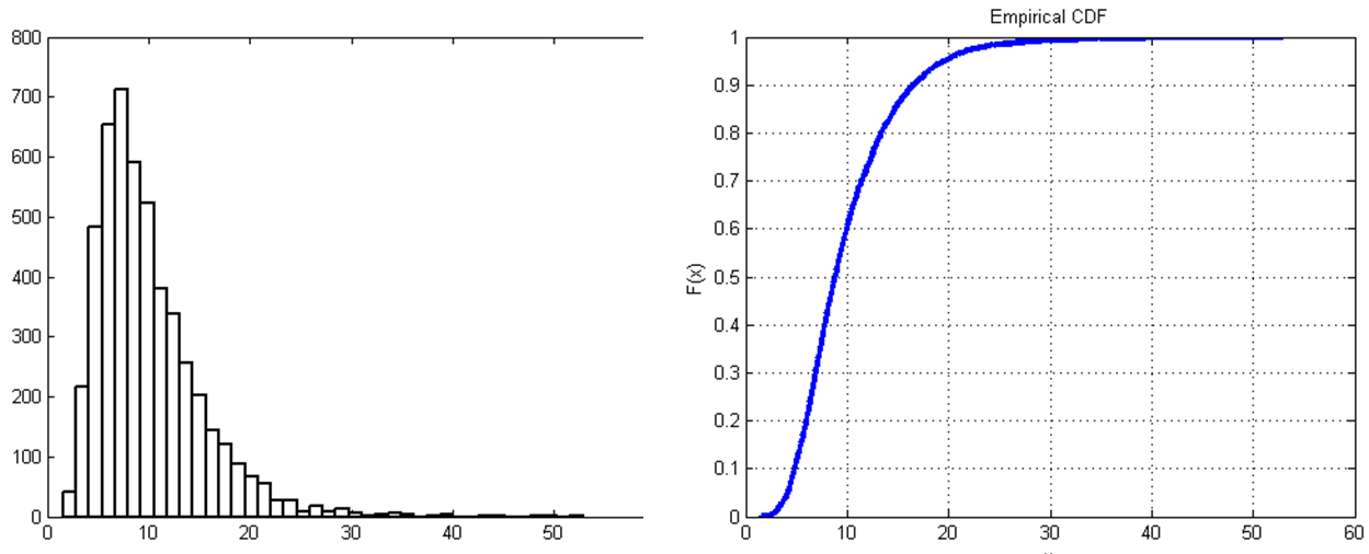
Figure 1.1: Sample patient treatment times and the corresponding empirical CDF.
In order to simulate the system, we need to understand and generate observations of these random variables as inputs to the model. Often, but not always, we have data from the real system that we use to characterize the input random variables. Typical outputs may include the patient waiting time, time in the system, and the care-giver and space utilizations. The simulation model will generate observations of these random variables. By controlling the execution of the simulation model, we can use the generated observations to characterize the outputs of interest. In the following section, we will discuss input and output analysis in the context of the general simulation process.
1.3.2 The Simulation Process
The basic simulation process is shown in Figure 1.2. Note that the process is not strictly sequential and will often turn out to be iterative. We will briefly discuss each of these components in the following paragraphs and will develop the topics in detail throughout the book.
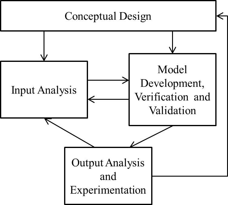
Figure 1.2: The simulation process.
Conceptual design requires a detailed understanding of the system being modeled as well as a basic modeling approach for creating the simulation model(s). Conceptual design can be done with pen and paper or on a whiteboard or similar collaboration space that promotes free thinking. It helps to be outside of the constraints of the simulation software package that you happen to be using. Although a well-defined process or methodology for conceptual design would be ideal, we do not know of one. Instead, planning the project is an informal process involving thinking about and discussing the details of the problem and the potential modeling approaches. Then the modelers can outline a systematic detailing of the modeling approach and decide on the application of software-specific details. Note that simulation models are developed for specific objectives and an important aspect of conceptual design is ensuring that the model will answer the questions being asked. In general, new simulationists (as well as new model builders in other domains) spend far too little time in the conceptual design phase. Instead, they tend to jump in and start the model development process. Allocating too little time for conceptual design almost always increases the overall time required to complete the project.
Input analysis (which is covered in detail in Chapter 6) involves characterizing the system inputs, and then developing the algorithms and computer code to generate observations on the input random variables and processes. Virtually all commercial simulation software (including Simio) has built-in features for generating the input observations. So the primary input-analysis task involves characterizing the input random variables and specifying corresponding distributions and processes to the simulation software. Often we have sample observations of the real-world data, and a common approach is is to fit standard or empirical distributions to these data that can then be used to generate the samples during the simulation (as show in Figure 1.1. Another approach is to randomly sample from the actual observed data. If we don’t have real-world data on inputs, we can use general rules-of-thumb and sensitivity analysis to help with the input-analysis task. In any of these approaches it is important to analyze the sensitivity of your model outputs to the selected inputs. Chapter 6 will also discuss the use of Input Parameters and how to use them to complete that analysis.
Model development is the coding process by which the conceptual model is converted into an executable simulation model. We don’t want to scare anybody off with the term coding — most modern simulation packages provide sophisticated graphical user interfaces to support modeling building/maintenance so the coding generally involves dragging and dropping model components and filling in dialog boxes and property windows. However, effective model development does require a detailed understanding of simulation methodology in general and how the specific software being used works in particular. The verification and validation steps ensure that the model is correct. Verification is the process that ensures that the model behaves as the developer intended, and the validation component ensures that the model is accurate relative to the actual system being modeled. Note that proving correctness in any but the simplest models will not be possible. Instead, we focus on collecting evidence until we (or our customers) are satisfied. Although this may disturb early simulationists, it is reality. Model development, verification, and validation topics are covered starting in Chapter 4 and throughout the remainder of the book.
Once a model has been verified and validated, you then exercise the model to glean information about the underlying system – this involves output analysis and experimentation. In the above examples, you may be interested in assessing performance metrics like the average time a patient waits before seeing a care-giver, the 90th percentile of the number of patients in the waiting room, the average number of vehicles waiting in the drive-through lane, etc. You may also be interested in making design decisions such as the number of care-givers required to ensure that the average patient waits no more than 30 minutes, the number of kitchen personnel to ensure that the average order is ready in 5 minutes, etc. Assessing performance metrics and making design decisions using a simulation model involves output analysis and experimentation. Output analysis takes the individual observations generated by the simulation, characterizes the underlying random variables (in a statistically valid way), and draws inferences about the system being modeled. Experimentation involves systematically varying the model inputs and model structure to investigate alternative system configurations. Output analysis topics are spread throughout the modeling chapters (4, 5, and 9).
1.4 When to Simulate (and When Not To)
Simulation of complicated systems has become quite popular. One of the main reasons for this is embodied in that word “complicated.” If the system of interest were actually simple enough to be validly represented by an exact analytical model, simulation wouldn’t be needed, and indeed shouldn’t be used. Instead, exact analytical methods like queueing theory, probability, or simple algebra or calculus could do the job. Simulating a simple system for which we can find an exact analytical solution only adds uncertainty to the results, making them less precise.
However, the world tends to be a complicated place, so we quickly get out of the realm of such very simple models. A valid model of a complicated system is likely be fairly complicated itself, and not amenable to a simple analytical analysis. If we go ahead and build a simple model of a complicated system with the goal of preserving our ability to get an exact analytical solution, the resulting model might be overly simple (simplistic, even), and we’d be uncertain whether it validly represents the system. We may be able to obtain a nice, clean, exact, closed-form analytical solution to our simple model, but we may have made a lot of simplifying assumptions (some of which might be quite questionable in reality) to get to our analytically-tractable model. We may end up with a solution to the model, but that model might not bear much resemblance to reality so we may not have a solution to the problem.
It’s difficult to measure how unrealistic a model is; it’s not even clear whether that’s a reasonable question. On the other hand, if we don’t concern ourselves with building a model that will have an analytical solution in the end, we’re freed up to allow things in the model to become as complicated and messy as they need to be in order to mimic the system in a valid way. When a simple analytically tractable model is not available, we turn to simulation, where we simply mimic the complicated system, via its complicated (but realistic) model, and study what happens to the results. This allows some model inputs to be stochastic — that is, random and represented by “draws” from probability distributions rather than by fixed constant input values — to represent the way things are in reality. The results from our simulation model will likewise be stochastic, and thus uncertain.
Clearly, this uncertainty or imprecision in simulation output is problematic. But, as we’ll, see, it’s not hard to measure the degree of this imprecision. If the results are too imprecise we have a remedy. Unlike most statistical sampling experiments, we’re in complete control of the randomness and number of replications, and can use this control to gain any level of precision desired. Computer time used to be a real barrier to simulation’s utility. But with modern software running on readily available fast, multi-processor computers and even cloud computing, we can do enough simulating to get results with imprecision that’s measurable, acceptably low, and perceptively valid.
In years gone by, simulation was sometimes dismissed as “the method of last resort,” or an approach to be taken only “when all else fails” ((Wagner 1969), pp. 887, 890). As noted above, simulation should not be used if a valid analytically-tractable model is available. But in many (perhaps most) cases, the actual system is just too complicated, or does not obey the rules, to allow for an analytically tractable model of any credible validity to be built and analyzed. In our opinion, it’s better to simulate the right model and get an approximate answer whose imprecision can be objectively measured and reduced, than to do an exact analytical analysis of the wrong model and get an answer whose error cannot be even be quantified, a situation that’s worse than imprecision.
While we’re talking about precise answers, the examples and figures in this text edition were created with Simio Version 17.261 (If you are using a newer version of Simio, look to the student area of the textbook web site where supplemental on-line content will be posted as it becomes available.). Because each version of Simio may contain changes that could affect low-level behavior (like the processing order of simultaneous events), different versions could produce different numerical output results for an interactive run. You may wonder “Which results are correct?” Each one is as correct (or as incorrect) as the others! In this book you’ll learn how to create statistically valid results, and how to recognize when you have (or don’t have) them. With the possible exception of a rare bug fix between versions, every version should generate statistically equivalent (and valid) results for the same model, even though they may differ numerically across single interactive runs.
1.5 Simulation Success Skills
Learning to use a simulation tool and understanding the underlying technology will not guarantee your success. Conducting successful simulation projects requires much more than that. Newcomers to simulation often ask how they can be successful in simulation. The answer is easy: “Work hard and do everything right.” But perhaps you want a bit more detail. Let’s identify some of the more important issues that should be considered.
1.5.1 Project Objectives
Many projects start with a fixed deliverable date, but often only a rough idea of what will be delivered and a vague idea of how it will be done. The first question that comes to mind when presented with such a challenge is “What are the project objectives?” Although it may seem like an obvious question with a simple answer, it often happens that stakeholders don’t know the answer.
Before you can help with objectives, you need to get to know the stakeholders. A stakeholder is someone who commissions, funds, uses, or is affected by the project. Some stakeholders are obvious — your boss is likely to be stakeholder (if you’re a student, your instructor is most certainly a stakeholder). But sometimes you have to work a bit to identify all the key stakeholders. Why should you care? In part because stakeholders often have differing (and sometimes conflicting) objectives.
Let’s say that you’re asked to model a specific manufacturing facility at a large corporation, and evaluate whether a new $4 million crane will provide the desired results (increases in product throughput, decreases in waiting time, reductions in maintenance, etc.). Here are some possible stakeholders and what their objectives might be in a typical situation:
Manager of industrial engineering (IE) (your boss): She wants to prove that IE adds value to the corporation, so she wants you to demonstrate dramatic cost savings or productivity improvement. She also wants a nice 3D animation she can use to market your services elsewhere in the corporation.
Production Manager: He’s convinced that buying a new crane is the only way he can meet his production targets, and has instructed his key people to provide you the information to help you prove that.
VP-Production: He’s been around a long time and is not convinced that this “simulation” thing offers any real benefit. He’s marginally supporting this effort due to political pressure, but fully expects (and secretly hopes) the project will fail.
VP-Finance: She’s very concerned about spending the money for the crane, but is also concerned about inadequate productivity. She’s actually the one who, in the last executive meeting, insisted on commissioning a simulation study to get an objective analysis.
Line Supervisor: She’s worked there 15 years and is responsible for material movement. She knows that there are less-expensive and equally effective ways to increase productivity, and would be happy to share that information if anyone bothered to ask her.
Materials Laborer: Much of his time is currently spent moving materials, and he’s afraid of getting laid off if a new crane is purchased. So he’ll do his best to convince you that a new crane is a bad idea.
Engineering Manager: His staff is already overwhelmed, so he doesn’t want to be involved unless absolutely necessary. But if a new crane is going to be purchased, he has some very specific ideas of how it should be configured and used.
This scenario is actually a composite of some real cases. Smaller projects and smaller companies might have fewer stakeholders, but the underlying principles remain the same. Conflicting objectives and motivations are not at all unusual. Each of the stakeholders has valuable project input, but it’s important to take their biases and motivations into account when evaluating their input.
So now that we’ve gotten to know the stakeholders a bit, we need to determine how each one views or contributes to the project objectives and attempt to prioritize them appropriately. In order to identify key objectives, you must ask questions like these:
What do you want to evaluate, or hope to prove?
What’s the model scope? How much detail is anticipated for each component of the system?
What components are critical? Which less-important components might be approximated?
What input information can be made available, how good is it, who will provide it, and when?
How much experimentation will be required? Will optimum-seeking be required?
How will any animation be used (animation for validation is quite different from animation presented to a board of directors)?
In what form do you want results (verbal presentation, detailed numbers, summaries, graphs, text reports)?
One good way to help identify clear objectives is to design a mock-up of the final report. You can say, “If I generate a report with the following information in a format like this, will that address your needs?” Once you can get general agreement on the form and content of the final report, you can often work backwards to determine the appropriate level of detail and address other modeling concerns. This process can also help bring out unrecognized modeling objectives.
Sometimes the necessary project clarity is not there. If so, and you go ahead anyway to plan the entire project including deliverables, resources, and date, you’re setting yourself up for failure. Lack of project clarity is a clear call to do the project in phases. Starting with a small prototype will often help clarify the big issues. Based on those prototype experiences, you might find that you can do a detailed plan for subsequent phases. We’ll talk more about that next.
1.5.2 Functional Specification
If you don’t know where you’re going, how will you know when you get there?
Carpenter’s advice: “Measure twice. Cut once.”
If you’ve followed the advice from Section 1.5.1, you now have at least some basic project objectives. You’re ready to start building the model, right? Wrong! In most cases your stakeholders will be looking for some commitments.
When will you get it done (is yesterday too soon)?
How much will it cost (or how many resources will it require)?
How comprehensive will the model be (or what specific system aspects will be included)?
What will be the quality (or how will it be verified and validated)?
Are you ready to give reliable answers to those questions? Probably not.
Of course the worst possible, but quite common, situation is that the stakeholder will supply answers to all of those questions and leave it to you to deliver. Picture a statement like “I’ll pay you $5000 to provide a thorough, validated analysis of … to be delivered five days from now.” If accepted, such a statement often results in a lot of overtime and produces an incomplete, unvalidated model a week or two late. And as for the promised money … well, the customer didn’t get what he asked for, now, did he?
It’s OK for the customer to specify answers to two of those questions, and in rare cases maybe even three. But you must reserve the right to adjust at least one or two of those parameters. You might cut the scope to meet a deadline. Or you might extend the deadline to achieve the scope. Or, you might double both the resources and the cost to achieve the scope and meet the date (adjusting the quality is seldom a good idea).
If you’re fortunate, the stakeholder will allow you to answer all four questions (of course, reserving the right to reject your proposal). But how do you come up with good answers? By creating a functional specification, which is a document describing exactly what will be delivered, when, how, and by whom. While the details required in a functional specification vary by application and project size, typical components may include the following:
Introduction
Simulation Objectives - Discussion of high-level objectives. What’s the desired outcome of this project?
Identification of stakeholders: Who are the primary people concerned with the results from this model? Which other people are also concerned? How will the model be used and by whom? How will they learn it?
System description and modeling approach: Overview of system components and approaches for modeling them including, but not limited to, the following components:
Equipment: Each piece of equipment should be described in detail, including its behavior, setups, schedules, reliability, and other aspects that might affect the model. Include data tables and diagrams as needed. Where data do not yet exist, they should be identified as such.
Product types: What products are involved? How do they differ? How do they relate to each other? What level of detail is required for each product or product group?
Operations: Each operation should be described in detail including its behavior, setups, schedules, reliability, and other aspects that might affect the model. Include data tables and diagrams as needed. Where data do not yet exist, they should be identified as such.
Transportation: Internal and external transportation should be described in adequate detail.
Input data: What data should be considered for model input? Who will provide this information? When? In what format?
Output data: What data should be produced by the model? In this section, a mock-up of the final report will help clarify expectations for all parties.
Project deliverables: Discuss all agreed-upon project deliverables. When this list is fulfilled, the project is deemed complete.
Documentation: What model documentation, instructions, or user manual will be provided? At what level of detail?
Software and training: If it’s intended that the user will interact directly with the model, discuss the software that’s required; what software, if any, will be included in the project price quote; and what, if any, custom interface will be provided. Also discuss what project or product training is recommended or will be supplied.
Animation: What are the animation deliverables and for what purposes will the animations be used (model validation, stakeholder buy-in, marketing)? 2D or 3D? Are existing layouts and symbols available, and in what form? What will be provided, by whom, and when?
Project phases: Describe each project phase (if more than one) and the estimated effort, delivery date, and charge for each phase.
Signoffs: Signature section for primary stakeholders.
At the beginning of a project there’s a natural inclination just to start modeling. There’s time pressure. Ideas are flowing. There’s excitement. It’s very hard to stop and do a functional specification. But trust us on this — doing a functional specification is worth the effort. Look back at those quotations at the beginning of this section. Pausing to determine where you’re going and how you’re going to get there can save misdirected effort and wasted time.
We recommend that approximately the first 10% of the total estimated project time be spent on creating a prototype and a functional specification. Do not consider this to be extra time. Rather, like in report design, you are just shifting some specific tasks to early in the project — when they can have the most planning benefit. Yes, that means if you expect the project may take 20 days, you should spend about two days on this. As a result, you may well find that the project will require 40 days to finish — certainly bad news, but much better to find out up front while you still have time to consider alternatives (reprioritize the objectives, reduce the scope, add resources, etc.).
1.5.3 Project Iterations
Simulation projects are best done as an iterative process, even from the first steps. You might think you could just define your objectives, create a functional specification, and then create a prototype. But while you’re writing the functional specification, you’re likely to discover new objectives. And while you’re doing the prototype, you’ll discover important new things to add to the functional specification.
As you get further into the project, an iterative approach becomes even more important. A simulation novice will often get an idea and start modeling it, then keep adding to the model until it’s complete — and only then run the model. But even the best modeler, using the best tools, will make mistakes. But when all you know is that your mistake is “somewhere in the model,” it’s very hard to find it and fix it. Based on our collective experience in teaching simulation, this is a huge problem for students new to the topic.
More experienced modelers will typically build a small piece of the model, then run it, test it, debug it, and verify that it does what the modeler expected it to do. Then repeat that process with another small piece of the model. As soon as enough of the model exists to compare to the real world, then validate, as much as possible, that the entire section of the model matches the intended system behavior. Keep repeating this iterative process until the model is complete. At each step in the process, finding and fixing problems is much easier because it’s very likely a problem in the small piece that was most recently added. And at each step you can save under a different name (like MyModelV1, MyModelV2, or with full dates and even times appended to the file names), to allow reverting to an earlier version if necessary.
Another benefit of this iterative approach, especially for novices, is that potentially-major problems can be eliminated early. Let’s say that you built an entire model based on a faulty assumption of how entity grouping worked, and only at the very end did you discover your misunderstanding. At that point it might require extensive rework to change the basis of your model. However, if you were building your model iteratively, you probably would have discovered your misunderstanding the very first time you used the grouping construct, at which time it would be relatively easy to take a better strategy.
A final, and extremely important benefit of the iterative approach is the ability to prioritize. For each iteration, work on the most important small section of the model that’s remaining. The one predictable thing about software development of all types is that it almost always takes much longer than expected. Building simulation models often shares that same problem. If you run out of project time when following a non-iterative approach and your model is not yet even working, let alone verified or validated, you essentially have nothing useful to show for your efforts. But if you run out of time when following an iterative approach, you have a portion of the model that’s completed, verified, validated, and ready for use. And if you’ve been working on the highest-priority task at each iteration, you may find that the portion completed is actually enough to fulfill most of the project goals (look up the 80-20 rule or the Pareto principle to see why).
Although it may vary somewhat by project and application, the general steps in a simulation study are:
Define high-level objectives and identify stakeholders.
Define the functional specification, including detailed goals, model boundaries, level of detail, modeling approach, and output measures. Design the final report.
Build a prototype. Update steps 1 and 2 as necessary.
Model or enhance a high-priority piece of the system. Document and verify it. Iterate.
Collect and incorporate model input data.
Verify and validate the model. Involve stakeholders. Return to step 4 as necessary.
Design experiments. Make production runs. Involve stakeholders. Return to step 4 as necessary.
Document the results and the model.
Present the results and collect your kudos.
As you’re iterating, don’t waste the opportunity to communicate regularly with the stakeholders. Stakeholders don’t like surprises. If the project is producing results that differ from what was expected, learn together why that’s happening. If the project is behind schedule, let stakeholders know early so that serious problems can be avoided. Don’t think of stakeholders as just clients, and certainly not as adversaries. Think of stakeholders as partners — you can help each other to obtain the best possible results from this project. And those results often come from the detailed system exploration that’s necessary to uncover the actual processes being modeled. In fact, in many projects a large portion of the value occurs before any simulation results are even generated — due to the knowledge gained from the early exploration by modelers, and frequent collaboration with stakeholders.
1.5.4 Project Management and Agility
There are many aspects to a successful project, but one of the most obvious is meeting the completion deadline. A project that produces results after the decision is made has little value. Other, often-related, aspects are the cost, resources, and time consumed. A project that runs over budget may be canceled before it gets close to completion. You must pay appropriate attention to completion dates and project costs. But both of those are outcomes of how you manage the day-to-day project details.
A well-managed project starts by having clear goals and a solid functional specification to guide your decisions. Throughout the project, you’ll be making large and small decisions, like the following:
How much detail should be modeled in a particular section?
How much input data do I need to collect?
To which output data should I pay most attention?
When is the model considered to be valid?
How much time should I spend on animation? On analysis?
What should I do next?
In almost every case, the functional specification should directly or indirectly provide the answers. You’ve already captured and prioritized the objectives of your key stakeholders. That information should become the basis of most decisions.
One of the things you’ll have to prioritize is evolving specifications or new stakeholder requests, sometimes called scope creep. One extreme is to take a hard line and say “If it’s not in the functional specification, it’s not in the model.” While in some rare cases this response may be appropriate and necessary, in most cases it’s not. Simulation is an exploratory and learning process. As you explore new areas and learn more about the target system, it’s only natural that new issues, approaches, and areas of study will evolve. Refusing to deal with these severely limits the potential value of the simulation (and your value as a solution provider).
Another extreme is to take the approach that the stakeholders are always right, and if they ask you to work on something new, it must be the right thing to do. While this response makes the stakeholder happy in the short-term, the most likely longer-term outcome is a late or even unfinished project — and a very unhappy stakeholder! If you’re always chasing the latest idea, you may never have the time to finish the high-priority work necessary to produce any value at all.
The key is to manage these opportunities — that management starts with open communication with the stakeholders and revisiting the items in the functional specification and their relative priorities. When something is added to the project, something else needs to change. Perhaps addressing the new item is important enough to postpone the project deadline a bit. If not, perhaps this new item is more important than some other task that can be dropped (or moved to the wish list that’s developed for when things go better than expected).
Our definition of agility is the ability to react quickly and appropriately to change. Your ability to be agile will be a significant contributor to your success in simulation.
1.5.5 Stakeholder and Simulationist Bills of Rights
We’ll end this chapter with an acknowledgment that stakeholders have reasonable expectations of what you will do for them (Figure 1.3). Give these expectations careful consideration to improve the effectiveness and success of your next project.
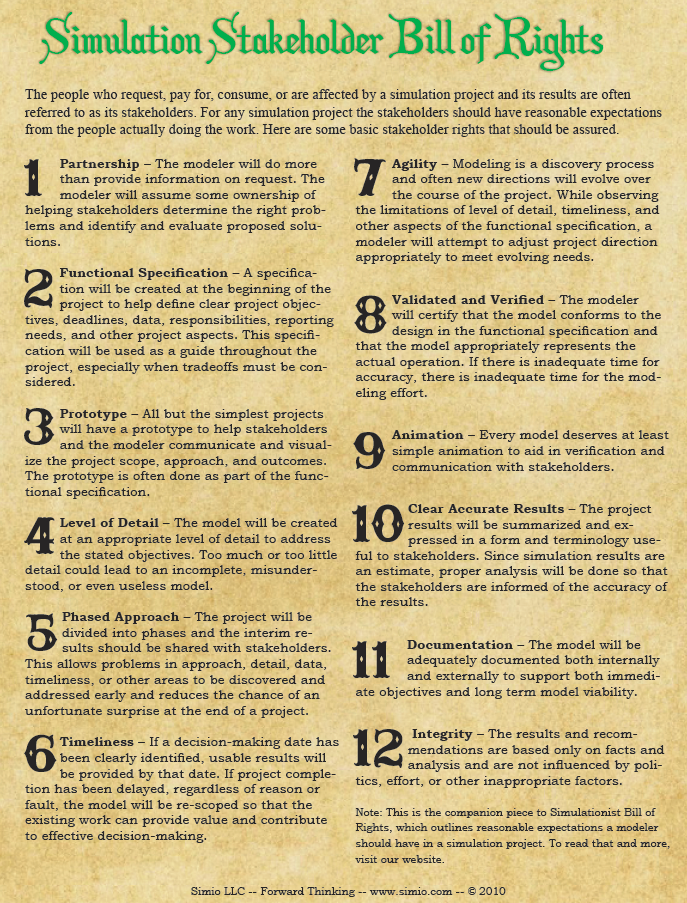
Figure 1.3: Simulation Stakeholder Bill of Rights.
But along with those expectations, stakeholders have some responsibilities to you as well (Figure 1.4). Discussing both sets of these expectations ahead of time can enhance communications and help ensure that your project is successful — a win-win situation that meets everyone’s needs. These rights were excerpted from the Success in Simulation (Sturrock 2012b) blog at www.simio.com/blog/ and used with permission. We urge you to peruse the early topics of this non-commercial blog for its many success tips and short interesting topics.
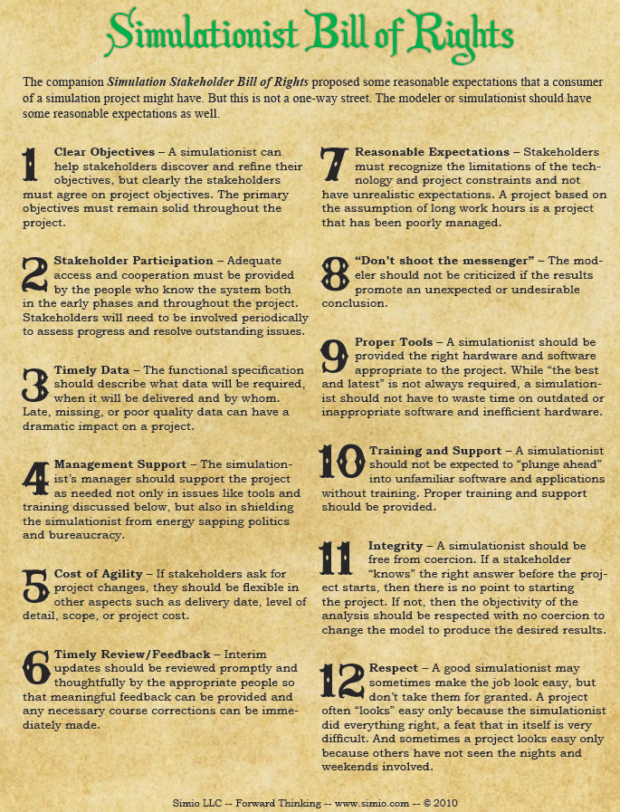
Figure 1.4: Simulationist Bill of Rights.