Simio and Simulation: Modeling, Analysis, Applications - 7th Edition
Chapter 3 Kinds of Simulation
Simulation is a very broad, diverse topic, and there are many different kinds of simulations, and approaches to carrying them out. In this chapter we describe some of these, and introduce terminology.
In Section 3.1 we classify the various kinds of simulations along several dimensions, and then in Section 3.2 we provide four examples of one kind of simulation, static stochastic (a.k.a. Monte Carlo) simulation. Section 3.3 considers two ways (manually and in a spreadsheet) of doing dynamic simulations without special-purpose dynamic-simulation software like Simio (neither is at all appealing, to say the least). Following that, Section 3.4 discusses the software options for doing dynamic simulations; Section 3.4.1 briefly describes how general-purpose programming languages like C++, Java, and Matlab might be used to carry out the kind of dynamic simulation logic done manually in Section 3.3.1, and Section 3.4.2 briefly describes special-purpose simulation software like Simio.
3.1 Classifying Simulations
Simulation is a wonderful word since it encompasses so many very different kinds of goals, activities, and methods. But this breadth can also sometimes render “simulation” a vague, almost-meaningless term. In this section we’ll delineate the different kinds of simulation with regard to model structure, and provide examples. While there are other ways to categorize simulations, it’s useful for us to consider static vs. dynamic; continuous-change vs. discrete-change (for dynamic models only); and deterministic vs. stochastic. Our focus in this book will be primarily on dynamic, discrete-change, stochastic simulation models.
3.1.1 Static vs. Dynamic Models
A static simulation model is one in which the passage of time plays no active or meaningful role in the model’s operation and execution. Examples are using a random-number generator to simulate a gambling game or lottery, or to estimate the value of an integral or the inverse of a matrix, or to evaluate a financial profit-and-loss statement. While there may be a notion of time in the model, unless its passage affects the model’s structure or operation, the model is static; three examples of this kind of situation, done via spreadsheets, are in Section 3.2.
In a dynamic simulation model, the passage of (simulated) time is an essential and explicit part of the model’s structure and operation; it’s impossible to build or execute the model without representing the passage of simulated time. Simulations of queueing-type systems are nearly always dynamic, since simulated time must be represented to make things like arrivals and service completions happen. An inventory simulation could be dynamic if there is logical linkage from one time to another in terms of, say, the inventory levels, re-stocking policy, or movement of replenishments. A supply-chain model including transportation or logistics would typically be dynamic since we’d need to represent the departure, movement, and arrival of shipments over time.
Central to any dynamic simulation is the simulation clock, just a variable representing the current value of simulated time, which is increased as the simulation progresses, and is globally available to the whole model. Of course, you need to take care to be consistent about the time units for the simulation clock. In modern simulation software, the clock is a real-valued variable (or, in computer-ese, a floating-point variable) so that the instants of time when things happen are represented exactly, or at least as exact as floating-point computer arithmetic can be (and that’s quite exact even if not perfect). We bring this up only because some older simulation software, and unfortunately still some current special-purpose simulator templates for things like combat modeling, require that the modeler select a small time step (or time slice or time increment), say one minute for discussion purposes here. The simulation clock steps forward in these time steps only, then stops and evaluates things to see if anything has happened to require updating the model variables, so in our example minute by minute. There are two problems with this. First, a lot of computer time can be burned by just this checking, at each minute boundary, to see if something has happened; if not then nothing is done and this checking effort is wasted. Secondly, if, as is generally true, things can in reality happen at any point in continuous time, this way of operating forces them to occur instead on the one-minute boundaries, which introduces time-distortion error into the model. True, this distortion could be reduced by choosing the time step to be a second or millisecond or nanosecond, but this just worsens the run-time problem. Thus, time-stepped models, or integer-valued clocks, have serious disadvantages, with no particular advantages in most situations.
Static simulations can usually be executed in a spreadsheet, perhaps facilitated via a static-simulation add-in like @Risk or Crystal Ball (Section 3.2), or with a general-purpose programming language like C++, Java, or Matlab. Dynamic simulations, however, generally require more powerful software created specifically for them. Section 3.3.1 illustrates the logic of what for us is the most important kind of simulation, dynamic discrete-change simulation, in a manual simulation that uses a spreadsheet to track the data and do the arithmetic (but is by no means any sort of general simulation model per se). As you’ll see in Section 3.3.2, it may be possible to build a general simulation model of a very, very simple queueing model in a spreadsheet, but not much more. For many years people used general-purpose programming languages to build dynamic simulation models (and still do on occasion, perhaps just for parts of a simulation model if very intricate nonstandard logic is involved), but this approach is just too tedious, cumbersome, time-consuming, and error-prone for the kinds of large, complex simulation models that people often want to build. These kinds of models really need to be done in dynamic-simulation software like Simio.
3.1.2 Continuous-Change vs. Discrete-Change Dynamic Models
In dynamic models, there are usually state variables that, collectively, describe the state of a simulated system at any point in (simulated) time. In a queueing system these state variables might include the lengths of the queues, the times of arrival of customers in those queues, and the status of servers (like idle, busy, or unavailable). In an inventory simulation the state variables might include the inventory levels and the amount of product on order.
If the state variables in a simulation model can change continuously over continuous time, then the model has continuous-change aspects. For example, the level of water in a tank (a state variable) can change continuously (i.e., in infinitesimally small increments/decrements), and at any point in continuous time, as water flows in the top and out the bottom. Often, such models are described by differential equations specifying the rates at which states change over time, perhaps in relation to their levels, or to the levels or rates of other states. Sometimes phenomena that are really discrete, like traffic flow of individual vehicles, are approximated by a continuous-change model, in this case viewing the traffic as a fluid. Another example of states that may, strictly-speaking, be discrete being modeled as continuous involves the famous Lanchester combat differential equations. In the Lanchester equations, \(x(t)\) and \(y(t)\) denote the sizes (or ) of opposing forces (perhaps the number of soldiers) at time \(t\) in the fight. There are many versions and variations of the Lanchester equations, but one of the simpler ones is the so-called modern (or aim-fire) model where each side is shooting at the other side, and the attrition rate (so a derivative with respect to time) of each side at a particular point in time is proportional to the size (level) of the other side at that time: \[\begin{equation} \begin{array}{l l} \dfrac{dx(t)}{dt} = -a y(t)\\[12pt] \dfrac{dy(t)}{dt} = -b x(t)\\ \end{array} \tag{3.1} \end{equation}\] where \(a\) and \(b\) are positive constants. The first equation in (3.1) says that the rate of change of the \(x\) force is proportional to the size of the \(y\) force, with \(a\) being a measure of effectiveness (lethality) of the \(y\) force — the larger the constant \(a\), the more lethal is the \(y\) force, so the more rapidly the \(x\) force is attritted. Of course, the second equation in (3.1) says the same thing about the simultaneous attrition of the \(y\) force, with the constant \(b\) representing the lethality of the \(x\) force. As given here, these Lanchester equations can be solved analytically, so simulation isn’t needed, but more elaborate versions of them cannot be analytically solved so would require simulation.
If the state variables can change only at instantaneous, separated, discrete points on the time axis, then the dynamic model is discrete-change. Most queueing simulation models are of this type, as state variables like queue lengths and server-status descriptors can change only at the times of occurrence of discrete events like customer arrivals, customer service completions, server breaks or breakdowns, etc. In discrete-change models, simulated time is realized only at the times of these discrete events — we don’t even look at what’s happening between successive events (because nothing is happening then). Thus, the simulation-clock variable jumps from the time of one event directly to the time of the next event, and at each of these points the simulation model must evaluate what’s happening, and what changes are necessary to the state variables (and to other kinds of variables we’ll describe in Section 3.3.1, like the event calendar and the statistical-tracking variables).
3.1.3 Deterministic vs. Stochastic Models
If all the input values driving a simulation model are fixed, non-random constants, then the model is deterministic. For example, a simple manufacturing line, represented by a queueing system, with fixed service times for each part, and fixed interarrival times between parts (and no breakdowns or other random events) would be deterministic. In a deterministic simulation, you’ll obviously get the same results from multiple runs of the model, unless you decide to change some of the input constants.
Such a model may sound a bit far-fetched to you, and it does to us too. So most simulation models are stochastic, where at least some of the input values are not fixed constants, but rather random draws (or random samples or random realizations) from probability distributions, perhaps characterizing the variation in service and interarrival times in that manufacturing line. Specifying these input probability distributions and processes is part of model building, and will be discussed in Chapter 6, where methods for generating these random draws from probability distributions and processes during the simulation will also be covered. Since a stochastic model is driven, at root, by some sort of random-number generator, running the model just once gives you only a single sample of what could happen in terms of the output — much like running the real (not simulated) production line for one day and observing production on that day, or tossing a die once and observing that you got a 4 on that toss. Clearly, you’d never conclude from that single run of the production line that what happened on that particular day is what will happen every day, or that the 4 from that single toss of the die means that the other faces of the die are also 4. So you’d want to run the production line, or toss the die, many times to learn about the results’ behavior (e.g., how likely it is that production will meet a target, or whether the die is fair or loaded). Likewise, you need to run a stochastic simulation model many times (or, depending on your goal, run it just once but for a very long time) to learn about the behavior of its results (e.g., what are the mean, standard deviation, and range of an important output performance measure?), a topic we’ll discuss in Chapters 4 and 5.
This randomness or uncertainty in the output from stochastic simulation might seem like a nuisance, so you might be tempted to eliminate it by replacing the input probability distributions by their means, a not-unreasonable idea that has sometimes been called mean-value analysis. This would indeed render your simulation output non-random and certain, but it might also very well render it wrong. Uncertainty is often part of reality, including uncertainty on the output performance metrics. But beyond that, variability in model inputs can often have a major impact on even the means of the output metrics. For instance, consider a simple single-server queue having exponentially distributed interarrival times with mean 1 minute, and exponentially distributed service times with mean 0.9 minute. From queueing theory (see Chapter 2), we know that in steady state (i.e., in the long run), the expected waiting time in queue before starting service is 8.1 minutes. But if we replaced the exponentially distributed interarrival and service times with their means (exactly 1 and 0.9 minute, respectively), it’s clear that there would never be any waiting in queue at all, so the mean waiting time in queue would be 0, which is very wrong compared to the correct answer of 8.1 minutes. Intuitively, variation in the interarrival and service times creates the possibility of many small interarrival times in a row, or many large service times in a row (or even just one really large service time), either of which leads to congestion and possibly long waits in queue. This is among the points made by Sam Savage in The Flaw of Averages: Why We Underestimate Risk in the Face of Uncertainty (Savage 2009).
It often puzzles people starting to use simulation software that executing your stochastic model again actually gets you exactly the same numerical results. You’d think this shouldn’t happen if a random-number generator is driving the model. But, as you’ll see in Chapter 6, most random-number generators aren’t really random at all, and will produce the same sequence of “random” numbers every time. What you need to do is replicate the model multiple times within the same execution, which causes you just to continue on in the fixed random-number sequence from one replication to the next, which will produce different (random) output from each replication and give you important information on the uncertainty in your results. Reproducibility of the basic random numbers driving the simulation is actually desirable for debugging, and for sharpening the precision of output by means of variance-reduction techniques, discussed in general simulation books like (Banks et al. 2005) and (Law 2015).
3.2 Static Stochastic Monte Carlo
Perhaps the earliest uses for stochastic computer simulation were in addressing models of systems in which there’s no passage of time, so there’s no time dimension at all. These kinds of models are sometimes called Monte Carlo, or stochastic Monte Carlo, a homage to the Mediterranean gambling paradise (or purgatory, depending on how you feel about gambling and casinos). In this section we’ll discuss four simple models of this kind. The first (Model 3-1) is the sum of throwing two dice. The second (Model 3-2) is using this kind of simulation to estimate the value of an analytically-intractable integral. The third (Model 3-3) is a model of a classical single-period perishable inventory problem. Finally, the fourth (Model 3-4) is a model that characterizes the expected profit of a proposed manufacturing project.
By the way, throughout this book, “Model \(x\)-\(y\)” will refer to the \(y\)th model in Chapter \(x\). The corresponding files, which can be downloaded as described in Appendix C, will be named Model_x_y.something, where the x and y will include leading zeros pre-pended if necessary to make them two digits, so that they’ll alphabetize correctly (we promise we’ll never have more than 99 chapters or more than 99 models in any one chapter). And something will be the appropriate file-name extension, like xls in this chapter for Excel files, and spfx later for Simio project files. Thus, Model 3-1, which we’re about to discuss, is accompanied by the file Model_03_01.xls.
We’ll use Microsoft ExcelR for the examples in this section due to its ubiquity and familiarity, but these kinds of simulations can also be easily done in programming languages like C++, Java, or Matlab.
3.2.1 Model 3-1: Throwing Two Dice
Throw two fair dice, and take the result as the sum of the faces that come up. Each die has probability \(1/6\) of producing each of the integers \(1, 2, ..., 6\) and so the sum will be one of the integers \(2, 3, ..., 12\). Finding the probability distribution of the sum is easy, and is commonly covered in books covering elementary probability, so there’s really no need to simulate this game, but we’ll do so anyway to illustrate the idea of static Monte Carlo.
In Model_03_01.xls (see Figure 3.1) we provide a simulation of this in Excel, and simulate 50 throws of the pair of dice, resulting in 50 values of the sum. All the possible face values are in cells C4..C9, the probabilities of each of the faces are in cells A4..A9, and the corresponding probabilities that the die will be strictly less than that face value are in cells B4..B9 (as you’ll see in a moment, it’s convenient to have these strictly-less-than probabilities in B4..B9 for generating simulated throws of each die). The throw numbers are in column E, the results of the two individual dice from each throw are in columns F and G, and their sum for each throw is in column H. In cells J4..L4 are a few basic summary statistics on the 50 sums. If you have the spreadsheet Model_03_01.xls open yourself (which we hope you do), you’ll notice that your results are different from those in Figure 3.1, since Excel’s random-number generator (discussed in the next paragraph) is what’s called volatile, so that it re-generates “fresh” random numbers whenever the spreadsheet is recalculated, which happens when it’s opened.
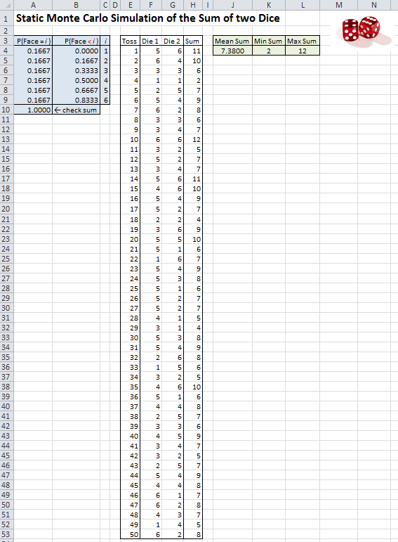
Figure 3.1: Static Monte Carlo simulation of throwing two fair dice.
The heart of this simulation is generating, or “simulating” the individual dice faces in cells F4..G53; we’ll discuss this in two steps. The first step is to note that Excel comes with a built-in random-number generator, RAND() (that’s right, the parentheses are required but there’s nothing inside them), which is supposed to generate independent observations on a continuous uniform distribution between 0 and 1. We say “supposed to” since the underlying algorithm is a particular mathematical procedure that cannot, of course, generate “true” randomness, but only observations that “appear” (in the sense of formal statistical-inference tests) to be uniformly distributed between 0 and 1, and appear to be independent of each other. These are sometimes called pseudo-random numbers, a mouthful, so we’ll just call them random numbers. We’ll have more to say in Chapter 6 about how such random-number generators work, but suffice it to say here that they’re complex algorithms that depend on solid mathematical research. Though the method underlying Excel’s RAND() has been criticized, it will do for our demonstration purposes here, but we might feel more comfortable with a better random-number generator such as those supplied with Excel simulation add-ins like Palisade Corporation’s @RISK(R) (www.palisade.com), or certainly with full-featured dynamic-simulation software like Simio.
The second step transforms a continuous observation, let’s call it \(U\), distributed continuously and uniformly on \([0, 1]\) from RAND(), into one of the integers \(1, 2, ..., 6\), each with equal probability \(1/6\) since the dice are assumed to be fair. Though the general ideas for generating observations on random variables (sometimes called random variates) is discussed in Chapter 6, it’s easy to come up with an intuitive scheme for our purpose here. Divide the continuous unit interval \([0, 1]\) into six contiguous subintervals, each of width \(1/6\): \([0, 1/6)\), \([1/6, 2/6)\), …, \([5/6, 1]\); since \(U\) is a continuous random variate it’s not important whether the endpoints of these subintervals are closed or open, since \(U\) will fall exactly on a boundary only with probability 0, so we don’t worry about it. Remembering that \(U\) is continuously uniformly distributed across \([0, 1]\), it will fall in each of these subintervals with probability equal to the subintervals’ width, which is \(1/6\) for each subinterval, and so we’ll generate (or return) a value 1 if it falls in the first subinterval, or a value 2 if it falls in the second subinterval, and so on for all six subintervals. This is implemented in the formulas in cells F4..G53 (it’s the same formula in all these cells),
\[\begin{equation*}
= VLOOKUP(RAND(), \$B\$4:\$C\$9, 2, TRUE).
\end{equation*}\]
This Excel function VLOOKUP, with its fourth argument set to TRUE, returns the value in the second column (that’s what the 2 is for in the third argument) of the cell range B4..C9 (the second argument) in the row corresponding to the values between which RAND() (the first argument) falls in the first column of B4..C9. (The $s in $B$4:$C$9 are to ensure that reference will continue to be made to these fixed specific cells as we copy this formula down in columns F and G.) So we’ll get C4 (which is 1) if RAND() is between B4 and B5, i.e. between 0 and 0.1667, which is our first subinterval of width (approximately) \(1/6\), as desired. If RAND() is not in this first subinterval, VLOOKUP moves on to the second subinterval, between B5 and B6, so between 0.1667 and 0.3333, and returns C5 (which is 2) if RAND() is between these two values, which will occur with probability \(0.3333 - 0.1667 = 1/6\) (approximately). This continues up to the last subinterval if necessary (i.e., if RAND() happened to be large, between 0.8333 and 1, a width of approximately \(1/6\)), in which case we get C9 (which is 6). If you’re unfamiliar with the VLOOKUP function, it might help to, well, look it up online or in Excel’s help.
The statistical summary results in J4..L4 are reasonable since we know that the range of the sum is 2 to 12, and the true expected value of the sum is 7. Since Excel’s RAND() function is volatile, every instance of it re-generates a fresh random number any time the spreadsheet is recalculated, which can be forced by tapping the F9 key (there are also other ways to force recalculation). So try that a few times and note how the individual dice values change, as does the mean of their sum in J4 (and occasionally even the min sum and max sum in K4 and L4).
This idea can clearly be extended to any discrete probability distribution as long as the number of possible values is finite (we had six values here), and for unequal probabilities (maybe for dice that are “loaded,” i.e., not “fair” with equal probabilities for all six faces). See Problem 1 for some extensions of this dice-throwing simulation.
3.2.2 Model 3-2: Monte-Carlo Integration
Say you want to evaluate the numerical value of the definite integral \(\int_a^b h(x) dx\) (for \(a < b\)), which is the area under \(h(x)\) between \(a\) and \(b\), but suppose that, due to its form, it’s hard (or impossible) to find the anti-derivative of \(h(x)\) to do this integral exactly, no matter how well you did in calculus. To simplify the explanation, let’s assume that \(h(x) \geq 0\) for all \(x\), but everything here still works if that’s not true. The usual way to approach this is numerically, dividing the range \([a, b]\) into narrow vertical subintervals, then calculating the area in the strip above each subinterval under \(h(x)\) by any of several approximations (rectangles, trapezoids, or fancier formulas), and then summing these areas. As the subintervals get more and more narrow, this numerical method becomes more and more accurate as an approximation of the true value of the integral. But it’s possible to create a static Monte Carlo simulation to get a statistical estimate of this integral or area.
To do this, first, generate a random variate \(X\) that’s distributed continuously and uniformly between \(a\) and \(b\). Again, general methods of variate generation are discussed in Chapter 6, but here again there’s easy intuition to lead to the correct formula to do this. Since \(U =\) RAND() is distributed continuously and uniformly between 0 and 1, if we “stretch” the range of \(U\) by multiplying it by \(b - a\), we’ll not distort the uniformity of its distribution, and will likewise “stretch” its range to be uniformly distributed between 0 and \(b-a\) (using the word “stretch” implies we’re thinking that \(b - a > 1\) but this all still works if \(b - a < 1\), in which case we should say “compress” rather than “stretch”). Then if we add \(a\), the range will be shifted right to \([a, b]\), still of width \(b - a\), as desired, and still it’s uniformly distributed on this range since this whole transformation is just linear (by saying “shifted right” we’re thinking that \(a > 0\), but this all still works if \(a < 0\), in which case we should say “shifted left” when we add \(a < 0\)).
Next, take the value \(X\) you generated in the preceding paragraph such that it’s continuously uniformly distributed on \([a, b]\), evaluate the function \(h\) at this value \(X\), and finally multiply that by \(b - a\) to get a random variate we’ll call \(Y = (b - a) h(X)\). If \(h\) were a flat (or constant) function, then no matter where \(X\) happened to fall on \([a, b]\), \(Y\) would be equal to the area under \(h\) between \(a\) and \(b\) (which is the integral \(\int_a^b h(x) dx\) we’re trying to estimate) since we’d be talking about just the area of a rectangle here. But if \(h\) were a flat function, you wouldn’t be doing all this in the first place, so it’s safe to assume that \(h\) is some arbitrary curve, and so \(Y\) will not be equal to \(\int_a^b h(x) dx\) unless we were very lucky to have generated an \(X\) to make the rectangle of width \(b - a\) and height \(h(X)\) equal to the area under \(h(x)\) over \([a, b]\). However, we know from the first mean-value theorem for integration of calculus that there exists (at least one) such “lucky” \(X\) somewhere between \(a\) and \(b\) so we could always hope. But better than hoping for extremely good luck would be to hedge our bets and generate (or simulate) a large number of independent realizations of \(X\), compute \(Y = (b - a) h(X)\), the area of a rectangle of width \(b - a\) and height \(h(X)\) for each one of them, and then average all of these rectangle-area values of \(Y\). You can imagine that some rectangle-area values of \(Y\) will be bigger than the desired \(\int_a^b h(x) dx\), while others will be smaller, and maybe on average they’re about right. In fact, it can be shown by basic probability, and the definition of the expected value of a random variable, that the expected value of \(Y\), denoted as \(E(Y)\) is actually equal to \(\int_a^b h(x) dx\); see Problem 3 for hints on how to prove this rigorously.
As a test example, let’s take \(h(x)\) to be the probability density function of a normal random variable with mean \(\mu\) and standard deviation \(\sigma > 0\), which is often denoted as \(\phi_{\mu, \sigma}(x)\), and is given by
\[
\phi_{\mu, \sigma}(x) = \frac{1}{\sigma \sqrt{2 \pi}}e^{-\frac{(x - \mu)^2}{2 \sigma^2}}
\]
for any real value of \(x\) (positive, negative, or zero). There’s no simple closed-form anti-derivative of \(\phi_{\mu, \sigma}(x)\) (which is why old-fashioned printed statistics books used to have tables of normal probabilities in the back or on the inside covers), so this will serve as a good test case for Monte-Carlo integration, and we can get a very accurate benchmark from those old normal tables (or from more modern methods, like Excel’s built-in NORMDIST function). Purely arbitrarily, let’s take \(\mu = 5.8\), \(\sigma = 2.3\), \(a = 4.5\), and \(b = 6.7.\)
In Model_03_02.xls (see Figure 3.2) we provide a simulation of this in Excel, and simulate 50 draws of \(X\) (denoted \(X_i\) for \(i = 1, 2, \ldots, 50\)) distributed continuously and uniformly between \(a = 4.5\) and \(b = 6.7\) (column E), resulting in 50 values of \((6.7 - 4.5)\phi_{5.8, 2.3}(X_i)\) in column F; we used Excel’s NORMDIST function to evaluate the density \(\phi_{5.8, 2.3}(X_i)\) in column F. We leave it to you to examine the formulas in columns E and F to make sure you understand them. The average of the 50 values in column F is in cell H4, and in cell I4 is the exact benchmark value using NORMDIST again. Tap the F9 key a few times to observe the randomness in the simulated results.
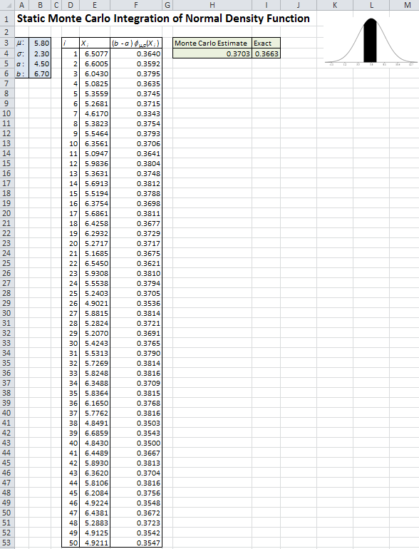
Figure 3.2: Static Monte Carlo integration of the normal density function.
Monte Carlo integration is seldom actually used for one-dimensional integrals like this, since the non-stochastic numerical area-estimating methods mentioned earlier are usually more efficient and quite accurate; Monte Carlo integration is, however, used to estimate integrals in higher dimensions, and over irregularly shaped domains of integration. See Problems 3 and 4 for analysis and extension of this example of Monte Carlo integration.
3.2.3 Model 3-3: Single-Period Inventory Profits
Your local sports team has just won the championship, so as the owner of several sporting-goods stores in the area you need to decide how many hats with the team’s logo you should order. Based on past experience, your best estimate of demand \(D\) within the next month (the peak period) is that it will be between \(a = 1000\) and \(b = 5000\) hats. Since that’s about all you think you can sell, you assume a uniform distribution; because hats are discrete items, this means that selling each of \(a = 1000, 1001, 1002, \ldots, 5000 = b\) hats is an event with probability \(1/(b+1-a) = 1/(5000 + 1 - 1000) = 1/4001 \approx 0.000249938\). Your supplier will sell you hats at a wholesale unit price of \(w = \$11.00\), and during the peak period you’ll sell them at a retail price of \(r = \$16.95\). If you sell out during the peak period you have no opportunity to re-order so you just miss out on any additional sales (and profit) you might have gotten if you’d ordered more. On the other hand, if you still have hats after the peak period, you mark them down to a clearance price of \(c = \$6.95\) and sell them at a loss; assume that you can eventually sell all remaining hats at this clearance price without further mark-downs. So, how many hats \(h\) should you order to maximize your profit?
Each hat you sell during the peak period turns a profit of \(r - w = \$16.95 - \$11.00 = \$5.95\), so you’d like to order enough to satisfy all peak-period demand. But each hat you don’t sell during the peak period loses you \(w - c = \$11.00 - \$6.95 = \$4.05\), so you don’t want to over-order either and incur this downside risk. Clearly, you’d like to wait until demand occurs and order just that many hats, but customers won’t wait and that’s not how production works, so you must order before demand is realized. This is a classical problem in the analysis of perishable inventories, known generally as the newsvendor problem (thinking of daily hardcopy newspapers [if such still exist when you read this book] instead of hats, which are almost worthless at the end of that day), and has other applications like fresh food, gardening stores, and even blood banks. Much research has investigated analytical solutions in certain special cases, but we’ll develop a simple spreadsheet simulation model that will be more generally valid, and could be easily modified to different problem settings.
We first need to develop a general formula for profit, expressed as a function of \(h =\) the number of hats ordered from the supplier. Now \(D\) is the peak-period demand, which is a discrete random variable distributed uniformly on the integers \(\{a=1000, 1001, 1002, \ldots, b=5000\}\). The number of hats sold at the peak-period retail price of \(r = \$16.95\) will be \(\min(D, h)\), and the number of hats sold at the post-peak-period clearance price of \(c = \$6.95\) will be \(\max(h-D, 0)\). To verify these formulas, try out specific values of \(h\) and \(D\), both for when \(D \ge h\) so you sell out, and for when \(D < h\) so you have a surplus left over after the peak period that you have to dump at the clearance price. Profit \(Z(h)\) is (total revenue) – (total cost):
\[\begin{equation} Z(h)\ \ = \underbrace{\underbrace{r \min(D, h)}_{\mbox{Peak-period revenue}} +\ \ \ \underbrace{c \max(h-D, 0)}_{\mbox{Clearance revenue}}}_{\mbox{Total revenue}}\ \ \ - \underbrace{w h}_{\mbox{Total cost}}. \end{equation}\] Note that the profit \(Z(h)\) is itself a random variable since it involves the random variable \(D\) as part of its definition; it also depends on the number of hats ordered, \(h\), so that’s part of its notation.
Before moving to the spreadsheet, there’s one more thing we need to figure out — how to generate (or “simulate”) observations on the demand random variable \(D\). We’ll again start with Excel’s built-in (pseudo)random-number generator RAND() to provide independent observations on a continuous uniform distribution between 0 and 1, as introduced earlier in Section 3.2.1. So for arbitrary integers \(a\) and \(b\) with \(a < b\) (in our example, \(a = 1000\) and \(b = 5000\)), how do we transform a random number \(U\) continuously and uniformly distributed between 0 and 1, to an observation on a discrete uniform random variable \(D\) on the integers \(\{a, a+1, ..., b\}\)? Chapter 6 discusses this, but for now we’ll just rely on some intuition, as we did for the two earlier spreadsheet simulations in Sections 3.2.1 and 3.2.2. First, \(a + (b + 1 - a)U\) will be continuously and uniformly distributed between \(a\) and \(b+1\); plug in the extremes \(U = 0\) and \(U = 1\) to confirm the range, and since this is just a linear transformation, the uniformity of the distribution is preserved. Then round this down to the next lower integer, an operation that’s sometimes called the integer-floor function and denoted \(\lfloor\cdot\rfloor\), to get
\[\begin{equation}
D = \lfloor a + (b + 1 - a)U \rfloor.
\tag{3.2}
\end{equation}\]
This will be an integer between \(a\) and \(b\) inclusively on both ends (we’d get \(D = b+1\) only if \(U = 1\), a probability-zero event that we can safely ignore). And the probability that \(D\) is equal to any one of these integers, say \(i\), is the probability that \(i \le a + (b + 1 - a)U < i+1\), which, after a bit of algebra, is the same thing as
\[\begin{equation}
\frac{i-a}{b+1-a} \le U < \frac{i+1-a}{b+1-a}.
\tag{3.3}
\end{equation}\]
Note that the endpoints are both on the interval \([0, 1]\). Since \(U\) is continuously uniformly distributed between 0 and 1, the probability of the event in the equation is just the width of this subinterval,
\[\begin{equation*}
\frac{i+1-a}{b+1-a} - \frac{i-a}{b+1-a} = \frac{1}{b+1-a} = \frac{1}{5000 + 1 - 1000} = \frac{1}{4001} \approx 0.000249938,
\end{equation*}\]
exactly as desired! Excel has an integer-floor function called INT, so the Excel formula for generating an observation on peak-period demand \(D\) is
\[\begin{equation}
= INT(a + (b + 1 - a)*RAND())
\tag{3.4}
\end{equation}\]
where \(a\) and \(b\) will be replaced by absolute references to the cells containing their numerical values (absolute since we’ll be copying this formula down a column).
The first sheet (tab at the bottom) of the file Model_03_03.xls contains our simulation using only the tools that come built-in with Excel. Figure 3.3 shows most of the spreadsheet (to save space, rows 27-54 are hidden and the numerical frequency-distribution tables at the bottom have been cropped out), but it’s best if you could just open the Excel file itself and follow along in it as you read, paying particular attention to the formulas entered in the cells.
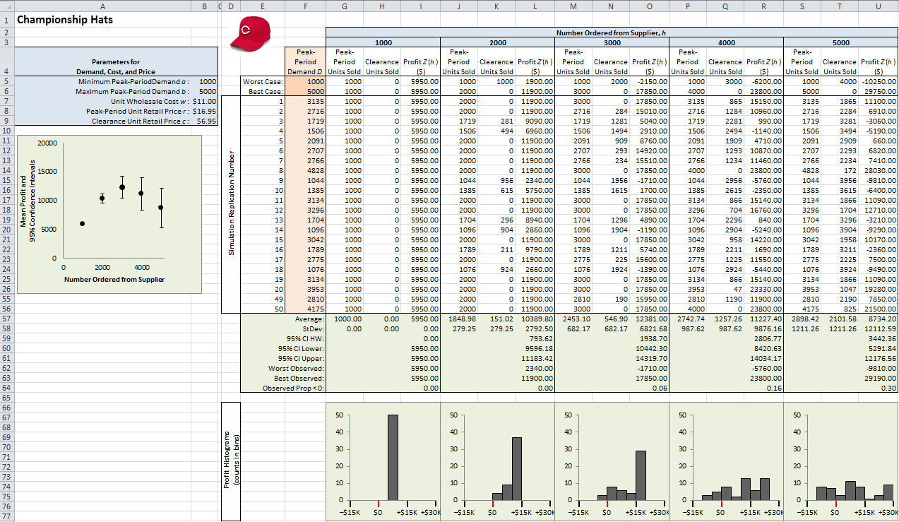
Figure 3.3: Single-period inventory spreadsheet simulation using only built-in Excel features.
The blue-shaded cells in A4..B9 contain the model input parameters. These should be set apart like this and then used in the formulas rather than “hard-wiring” these constants into the Excel model, to facilitate possible “what-if” experiments later to measure the impact of changing their values; that way, we need only change their values in the blue cells, rather than throughout the spreadsheet wherever they’re used. We decided, essentially arbitrarily, to make 50 IID replications of the model (each row is a replication), and the replication number is in column E. Starting in row 7 and going down, the light-orange-shaded cells in Column F contain the 50 peak-period demands \(D\),
which in each of these cells is the formula
\[\begin{equation*}
=INT(\$B\$5 + (\$B\$6 + 1 - \$B\$5)*RAND())
\end{equation*}\]
since \(a\) is in B5 and \(b\) is in B6. We use the \$ symbols to force these to be absolute references since we typed this formula into F7 and then copied it down. Above the realized demands, we entered the worst possible (\(a = 1000\)) and best possible (\(b = 5000\)) cases for peak-period demand \(D\) in order to see the worst and best possible values of profit for each trial value of \(h =\) number of hats ordered, as well as the 50 realized values of profit for each of the 50 realized values of peak-period demand \(D\) and for each trial value of \(h\). If you have this spreadsheet open you’ll doubtless see numerical results that differ from those in Figure 3.3 because Excel’s RAND() function is volatile, meaning that it re-generates every single random number in the spreadsheet upon each spreadsheet recalculation. One way to force a recalculation is to tap the F9 key on your keyboard, and you’ll see all the numbers (and the plots) change. Even though we have 50 replications, there is still considerable variation from one set of 50 replications to the next, with each tap of the F9 key. This only serves to emphasize the importance of proper statistical design and analysis of simulation experiments, and to do something to try to ascertain an adequate sample size.
We took the approach of simply trying several values for \(h\) (1000, 2000, 3000, 4000, and 5000) spanning the range of possible peak-period demands \(D\) under our assumptions. For each of these values of \(h\), we computed the profit on each of the 50 replications of peak-period demand if \(h\) had been each of these values, and then summarized the statistics numerically and graphically.
If we order just \(h = 1000\) hats (columns G-I), then we sell 1000 hats at the peak-period price for sure since we know that \(D \ge 1000\) for sure, leading to a profit of exactly \((r - w)D = (\$16.95 - \$11.00)\times 1000 = \$5950\) every time — there’s no possibility of having anything left over to dump at the clearance price (column H contains only 0s), and there’s no risk of profiting any less than this. There’s also no chance of profiting any more than this $5950 since, of course, if \(D > 1000\), which it will be with very high probability (\(1 - 1/(5000 + 1 - 1000) \approx 0.999750062\)), you’re leaving money on the table with such a small, conservative, totally risk-averse choice of \(h\).
Moving further to the right in the spreadsheet, we see that for higher order values \(h\), the mean profits (row 57) rise to a maximum point at somewhere around \(h = 3000\) or 4000, then fall off for \(h = 5000\) due to the relatively large numbers of hats left unsold after the peak period; this is depicted in the plot in column A where the heavy dots are the sample means and the vertical I-beams depict 95% confidence intervals for the population means. As \(h\) rises there is also more variation in profit (look at the standard deviations in row 58), since there is more variation in both peak-period units sold and clearance units sold (note that their sum is always \(h\), which it of course must be in this model). This makes the 95% confidence intervals on expected profit (rows 59-61 and the plot in column A) larger, and also makes the histograms of profit (rows 66-77) more spread out (it’s important that they all be scaled identically), which is both good and bad — the good is that there’s a chance, albeit small, to turn very large profits; but the bad is that there’s an increasing chance of actually losing money (row 64, and the areas to the left of the red zero marker in the histograms). So, how do you feel about risk, both upside and downside?
The second sheet of Model_03_03.xls has the same simulation model but using the simulation add-in @RISK from Palisade Corporation; see Figure 3.4 with the @RISK ribbon showing at the top, but again it’s better if you just open the file to this sheet. To execute (or even properly view) this sheet you must already have @RISK loaded – see Section C.4.4 for information on obtaining the software and watching introductory videos. We won’t attempt here to give a detailed account of @RISK, as that’s well documented elsewhere, e.g. (Albright, Winston, and Zappe 2009). But here are the major points and differences from simulating using only the built-in Excel capabilities:
We still have to create the basic model, the most important parts of which are the input (blue-shaded) areas, and the formulas in row 7 for the outputs (profits in this model).
However, we no longer need to copy this single-row simulation down to many more rows, one for each replication.
@RISK provides the capability for a large number of input distributions, including the discrete uniform we want for peak-period demands. This is entered in cell F7 via the @RISK formula
=RiskIntUniform(1000,5000), which can be entered by first single-clicking in this cell, and then clicking the Define Distributions button on the left end of the @RISK ribbon to find a gallery of distributions from which to select and parameterize your inputs (we have only one random input in this model).The number of replications (or ``Iterations’’ as they’re called by @RISK) is simply entered (or selected from the pull-down) in that field near the center of the @RISK ribbon. We selected 1000, which is the same thing as having 1000 explicit rows in our original spreadsheet simulation using only the built-in Excel tools.
We need to identify the cells that represent the outputs we want to watch; these are the profit cells I7, L7, O7, R7, and U7. To do so, just click on these cells, one by one, and then click the
Add Outputbutton near the left end of the @RISK ribbon and optionally change the Name for output labeling. We’ve shaded these cells light green.To run the simulation, click the
Start Simulationbutton just to the right of the Iterations field in the @RISK ribbon.We don’t need to do anything to collect and summarize the output (as we did before with the means, confidence intervals, and histograms) since @RISK keeps track of and summarizes all this behind the scenes.
There are many different ways to view the output from @RISK. Perhaps one of the most useful is an annotated histogram of the results. To get this (as shown in Figure 3.4), single-click on the output cell desired (such as R7, profit for the case of \(h = 4000\)), then click on the Browse Results button in the @RISK ribbon. You can drag the vertical splitter bars left and right and get the percent of observations between them (like 15.6% negative profits, or losses, in this case), and in the left and right tails beyond the splitter bars. Also shown to the right of the histogram are some basic statistics like mean, standard deviation, minimum, and maximum.
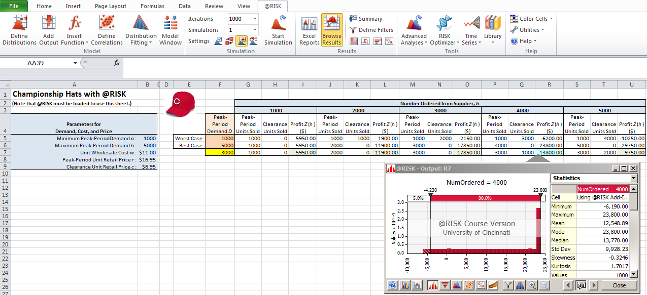
Figure 3.4: Single-period inventory spreadsheet simulation using Palisade add-in.
It’s clear that add-ins like @RISK greatly ease the task of carrying out static simulations in spreadsheets. Another advantage is that they provide and use far better random-number generators than the RAND() function that comes with Excel. Competing static-simulation add-ins for Excel include Oracle’s Crystal BallTM (www.oracle.com/crystalball/), and Frontline Systems’ Risk SolverTM (www.solver.com/risk-solver-pro).
3.2.4 Model 3-4: New Product Decision Model
This section presents a Monte Carlo model that characterizes the expected profit of a project involving producing and selling a new product. We present two implementations of this model – one using Excel, similar to the previous models in this chapter, and another using a programmatic approach implemented in Python. This problem is based on a similar problem defined by Anthony Sun (originally used with permission1) in which a company is considering manufacturing and marketing a new product and would like to predict the potential profit associated with the product.
The total profit of the project is given by the total revenue from sales minus the total cost to manufacture and is given by the equation:
\[\begin{equation} TP=(Q \times P)-(Q \times V+F) \tag{3.5} \end{equation}\]
where \(TP\) is the total profit, \(Q\) is the quantity sold, \(P\) is the selling price, \(V\) is the variable (marginal) cost, and \(F\) is the fixed cost for setting up the production facilities. Note that we are ignoring the time-value of money and other factors in order to simplify the model, but these could easily be added to improve the model realism. Since the firm is predicting what will happen if they produce the product in the future, some of the profit equation components are uncertain. In particular, \(Q\), \(P\), and \(V\) are assumed to be random variables with the following distributions:
- \(Q \sim \textrm{Uniform}(10000, 15000)\)
- \(P \sim 1 + \textrm{Lognormal}(3.75, 0.65)\)
- \(V \sim 12 + \textrm{Weibull}(10)\)
and \(F\) is fixed at \(\$150,000\). The ultimate question to be answered is whether the firm should undertake the project of producing and selling the new project. Since \(Q\), \(P\), and \(V\) are random variables, the total profit, \(TP\) will also be a random variable. In order to assist the decision-maker at the firm, we would like to estimate the probability distribution for this random variable. Using this distribution, we can then estimate parameters of interest, including the mean, standard deviation, and percentiles of the profit.
Figure 3.5 illustrates the distributions for \(Q\), \(P\), and \(V\), respectively, using histograms based on \(250,000\) samples from each of the “actual” distributions. A natural question here is “Where do these distributions come from?” While it is possible that a firm might have historical data to which to fit probability distributions (see Section 6.1), it is more likely that someone or some group with domain expertise estimated them. In our case, we wanted to model significant uncertainty in the quantity sold – the uniform distribution would be akin to saying, “somewhere between \(10,000\) and \(15,000\),” with no additional information. To the extent that the selling price is largely determined by the market, we also wanted uncertainty there, but feel that it would have more of a central tendency and wanted to allow the possibility that the product would be a huge hit (so would command a high selling price), or a miserable flop (so the company would be forced to lower the selling price near 1, which is the minimum of the lognormal distribution specified). Finally, we feel confident that the firm would have better control over the variable cost, but wanted some uncertainty to account for factors such as raw material and labor cost. The selected lognormal and Weibull distributions provide these general shape characteristics.
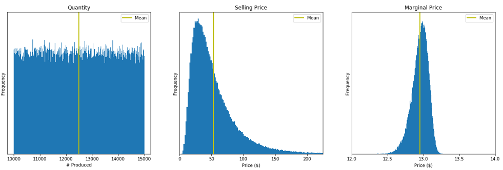
Figure 3.5: Samples from the distributions of Q, P, and V, respectively, generated from the Python version of Model 3-4.
As with our previous Monte Carlo examples, our process will involve sampling observations for each of these random variables and then using the equation to compute the corresponding sample of the total profit random variable and then replicating this process. The pseudo-code for our Monte Carlo model is shown in Algorithm 1 (note that we rearranged it to reduce the computational requirement).
Algorithm 1 - Sample TP
n = 250,000
F = 150,000
tp = []
FOR{i = 1 to n}
sample P
sample V
sample Q
profit = Q(P-V)-F
tp.append(profit)
ENDFOR
Upon execution of the corresponding code/model, \(tp\) will be a list/array of the sampled observations of total profit and we can use the values to estimate the distribution parameters of interest.
Sampling the observations of \(Q\), \(P\), and \(V\) is the critical part of Algorithm 1 and the algorithm can be easily implemented using any tool/language that supports the generation of observations from these random variables (as we’ll explain in Section 6.4, we call such observations random variates). The general topic of random variate generation is covered in Section 6.4, but for our Excel and Python versions of Model 3-4, we will just use the formulae/functions shown in Figure 3.6 (see Sections 6.3 and 6.4 for why these formulae are valid). \(L\) and \(U\) are the lower and upper limits for the uniform distribution, \(mu\) and \(sigma\) are the mean and standard deviation of the normal distribution used for the lognormal random variables, \(alpha\) is the shape parameter of the Weibull distribution, and \(n\) is the number of observations to generate.
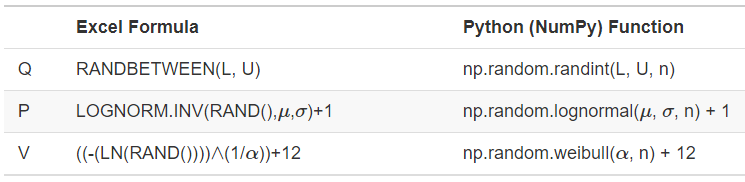
Figure 3.6: Formulae and functions for generating observations of \(Q\), \(P\), and \(V\) for Model 3-4.
Figure 3.7 shows the computational portion of the Python version of Model 3-4 along with the generated histogram total profit (\(TP\)) based on \(250,000\) replications.
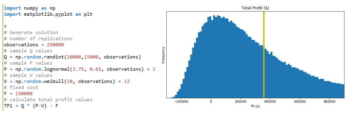
Figure 3.7: The computational portion of the Python version of Model 3-4 and the histogram of total profit.
Figure 3.8 shows a portion of the Excel version of Model 3-4 (which uses 100,000 replications). Both versions of the model generate the array of observations of total profit as described in Algorithm 1 and then computes summary and descriptive statistics and generates the histogram that estimates the probability distribution.
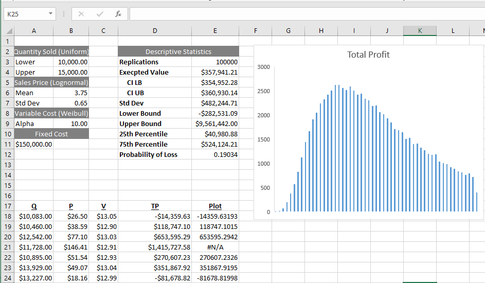
Figure 3.8: The Excel version of Model 3-4.
Armed with the results of the runs of Model 3-4 we are ready to address the original question posed – Should the firm undertake the project? The descriptive statistics and histogram (shown in Figures 3.8 and 3.7) provide useful information. While the expected profit is approximately $\(360,000\), there is also an approximate \(19\%\) chance of actually losing money. In addition, the standard deviation ($\(482,000\)) and the 25th and 75th percentiles ($\(41,000\) and $\(524,000\), respectively) provide additional information about the risk of undertaking the project. Chapter 4 goes further into the concepts of risk and error in this context. Of course the actual decision of whether to undertake the project would depend on the firm’s risk tolerance, expected return on capital, other opportunities, etc., but it is clear that the information provided by the model would be useful input for the decision maker.
3.3 Dynamic Simulation Without Special Software
In this section we’ll consider how dynamic simulations might be carried out without the benefit of special-purpose dynamic-simulation software like Simio. Section 3.3.1 carries out a manual (i.e., no computer at all) simulation of a simple single-server queue, using an Excel spreadsheet to help with the record-keeping and arithmetic, but that is by no means any kind of general manual-simulation ``model.’’ Then Section 3.3.2 develops a spreadsheet model of part of a single-server queue by exploiting a very special relationship that is not available for more complex dynamic queueing simulations.
3.3.1 Model 3-5: Manual Dynamic Simulation
Though you won’t see it using high-level simulation-modeling software like Simio, all dynamic discrete-change simulations work pretty much the same way under the hood. In this section we’ll describe how this goes, since even with high-level software like Simio, it’s still important to understand these concepts even if you’ll (thankfully) never actually have to do a simulation this way. The logic for this is also what you’d need to code a dynamic discrete-change simulation using a general-purpose programming language like C++, Java, or Matlab.
Our system here is just a simple single-server queue. Entities (which could represent customers in a service system, parts in a manufacturing system, or patients in a health-care system) show up at arrival times that, for now, will be assumed to be simply given from some magical (see Section 4.2.1) outside source (we’ll assume the first arrival to be at time 0), and require service times that are also just given; all times are in minutes and the queue discipline is first-in, first-out (FIFO). The simulation will just end abruptly at time 8 minutes, even if entities are in queue or in service at that time. For output, we’ll compute the utilization of the server (proportion or percent of time busy), as well as the average, minimum, and maximum of each of (a) the total entity time in system, (b) the entity time in queue (just waiting in line, exclusive of service time), (c) the number of entities in the system, and (d) the number of entities in the queue. The averages in (a) and (b) are just simple averages of lists of numbers, but the averages in (c) and (d) are time-averages, which are the total areas under the curves tracking these variables over continuous time, divided by the final simulation-clock time, 8. For example, if \(L_q(t)\) is the number of entities waiting in the queue at time \(t\), then the time-average number of entities in queue is \(\int_0^8 L_q(t)dt/8\), which is just the weighted average of the possible queue-length values (\(0, 1, 2, \ldots\)), with the weights being the proportions of time the curve is at level \(0, 1, 2, \ldots\). Likewise, if \(B(t)\) is the server-busy function (0 if idle at time \(t\), 1 if busy at time \(t\)), and \(L(t)\) is the number of entities in system (in queue plus in service) at time \(t\), then the server-utilization proportion is \(\int_0^8 B(t)dt/8\), and the time-average number of entities in system is \(\int_0^8 L(t)dt/8\).
We’ll keep track of things, and do the arithmetic, in an Excel spreadsheet called Model_03_05.xls, with the files that accompany this book and can be downloaded as described in Appendix C, shown in Figure 3.9. The spreadsheet holds the data and does calculations. The pink-shaded cells contain formulas that are specific to this particular input set of arrival and service times, so this spreadsheet isn’t a general model per se that will work for any set of arrival and service times.The light-blue-shaded cells B5..B14 and D5..D14 contain the given arrival and service times. It turns out to be more convenient to work with – rather than the given arrival times – the interarrival times, which are calculated via the Excel “=” formulas in C6..C14; type “CTRL-`” (while holding down the Control key, type the backquote character) to toggle between viewing the values and formulas in all cells. Note that an interarrival time in a row is the time between the arrival of that row’s entity and the arrival of the prior entity in the preceding row (explaining why there’s no interarrival time for entity 1, which arrives at time 0).
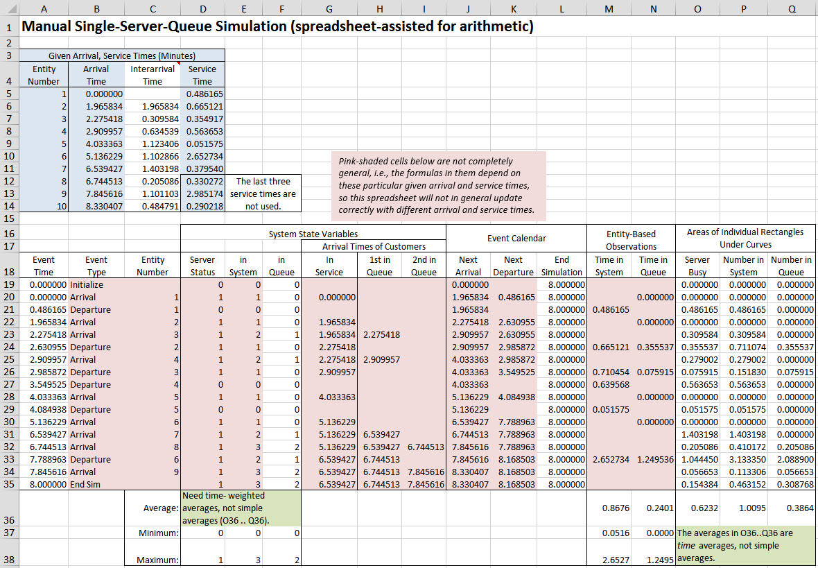
Figure 3.9: Manual discrete-change simulation of a single-server queue.
In a dynamic discrete-change simulation, you first identify the events that occur at instants of simulated time, and that may change the system state. In our simple single-server queue, the events will be the arrival of an entity, the end of an entity’s service and immediate departure from the system, and the end of the simulation (which might seem like an “artificial” event but it’s one way to stop a simulation that’s to run for a fixed simulated-time duration — we’ll “run” ours for 8 minutes). In more complex simulations, additional events might be the breakdown of a machine, the end of that machine’s repair time, a patient’s condition improves from one acuity level to a better one, the time for an employee break rolls around, a vehicle departs from an origin, that vehicle arrives at its destination, etc. Identifying the events in a complex model can be difficult, and there may be alternative ways to do so. For instance, in the simple single-server queue you could introduce another event, when an entity begins service. However, this would be unnecessary since this “begin-service” event would occur only when an entity ends service and there are other entities in queue, or when a lucky entity arrives to find the server idle with no other entities already waiting in line so goes directly into service; so, this “event” is already covered by the arrival and departure events.
As mentioned in Section 3.1.2, the simulation clock in a dynamic discrete-change model is a variable that jumps from one event time to the next in order to move the simulation forward. The event calendar (or event list) is a data structure of some sort that contains information on upcoming events. While the form and specific type of data structure vary, the event calendar will include information on when in simulated time a future event is to occur, what type of event it is, and often which entity is involved. The simulation proceeds by identifying the next (i.e., soonest) event in the event calendar, advancing the simulation-clock variable to that time, and executing the appropriate event logic. This effects all the necessary changes in the system state variables and the statistical-tracking variables needed to produce the desired output, and updates the event calendar as required.
For each type of event, you need to identify the logic to be executed, which sometimes depends on the state of the system at the moment. Here’s basically what we need to do when each of our event types happens in this particular model:
- Arrival First, schedule the next arrival for now (the simulation-clock value in Column A) plus the next interarrival time in the given list, by updating the next-arrival spot in the event calendar (column J in
Model_03_05.xlsand Figure 3.9. Compute the continuous-time output areas of the rectangles under \(B(t)\), \(L(t)\), and \(L_q(t)\) between the time of the last event and now, based on their values that have been valid since that last event and before any possible changes in their values that will be made in this event; record the areas of these rectangles in columns O-Q. What we do next depends on the server status:- If the server is idle, put the arriving entity immediately into service (put the time of arrival of the entity in service in the appropriate row in column G, to enable later computation of the time in system), and schedule this entity’s service completion for now plus the next service time in the given list. Also, record into the appropriate row in column N a time in queue of 0 for this lucky entity.
- If the server is busy, put the arriving entity’s arrival time at the end of a list representing the queue of entities awaiting service, in the appropriate row of columns H-I (it turns out that the queue length in this particular simulation is never more than two, so we need only two columns to hold the arrival times of entities in queue, but clearly we could need more in other cases if the queue becomes longer). We’ll later need these arrival times to compute times in queue and in system. Since this is the beginning of this entity’s time in queue, and we don’t yet know when it will leave the queue and start service, we can’t yet record a time in queue into Column N for this entity.
- Departure. (upon a service completion). As in an arrival event, compute and record the continuous-time output areas since the last event in the appropriate row of columns O-Q. Also, compute and record into the appropriate row in column M the time in system of the departing entity (current simulation clock, minus the time of arrival of this entity, which now resides in column G). What we do next depends on whether there are other entities waiting in queue:
- If other entities are currently waiting in the queue, take the first entity out of queue and place it into service (copy the arrival time from column H into the next row down in column G). Schedule the departure of this entity (column K) for now plus the next service time. Also compute the time in queue of this entity (current simulation clock in column A, minus the arrival time just moved into column G) into the appropriate row in column N.
- If there are no other entities waiting in queue, simply make the server-status variable (column D below row 18) 0 for idle, and blank out the event-calendar entry for the next departure (column K).
- End simulation (at the fixed simulation-clock time 8 minutes). Compute the final continuous-time output areas in columns O-Q from the time of the last event to the end of the simulation, and compute the final output summary performance measures in rows 36-38.
It’s important to understand that, though processing an event will certainly take computer time, there is no simulation time that passes during an event execution — the simulation-clock time stands still. And as a practical matter in this manual simulation, you probably should check off in some way the interarrival and service times as you use them, so you can be sure to move through the lists and not skip or re-use any of them.
Rows 19-35 of the spreadsheet Model_03_05.xls and in Figure 3.9 trace the simulation from initialization at time 0 (row 19), down to termination at time 8 minutes (row 35), with a row for each event execution. Column A has the simulation-clock time \(t\) of the event, column B indicates the event type, and column C gives the entity number involved. Throughout, the cell entries in a row represent the appropriate values after the event in that row has been executed, and blank cells are places where an entry isn’t applicable. Columns D-F give respectively the server status \(B(t)\) (0 for idle and 1 for busy), the number of entities in the system, and the number of entities in the queue (which in this model is always the number in system minus the server status … think about it for a minute). Column G contains the time of arrival of the entity currently in service, and columns H-I have the times of arrival in the first two positions in the queue (we happen never to need a queue length of more than two in this example).
The event calendar is in columns J-L, and the next event is determined by taking the minimum of these three values, which is what the =MIN function in column A of the following row does. An alternative data structure for the event calendar is to have a list (or more sophisticated data structure like a tree or heap) of records or rows of the form [entity number, event time, event type], and when scheduling a new event insert it so that you keep this list of records ranked in increasing order on event time, and thus the next event is always at the top of this list. This is closer to the way simulation software actually works, and has the advantage that we could have multiple events of the same type scheduled, as well as being much faster (especially when using the heap data structure), which can have a major impact on run speed of large simulations with many different kinds of events and long event lists. However, the simple structure in columns J-L will do for this example.
When a time in system is observed (upon a departure), or a time in queue is observed (upon going into service), the value is computed (the current simulation clock in column A, minus the time of arrival) and recorded into column M or N. Finally, columns O-Q record the areas of the rectangles between the most recent event time and the event time of this row, in order to compute the time averages of these curves.
The simulation starts with initialization in row 19 at time 0. This should be mostly self-explanatory, except note that the end-simulation event time in L19 is set for time 8 minutes here (akin to lighting an 8-minute fuse), and the next-departure time is left blank (luckily, Excel interprets this blank as a large number so that the =MIN in A20 works).
The formula =MIN(J19:L19) in A20 finds the smallest (soonest) value in the event calendar in the preceding row, which is 0, signifying the arrival of entity 1 at time 0. We change the server status to 1 for busy in D20, and the number in system is set to 1 in E20; the number in queue in F20 remains at 0. We enter 0 in G20 to record the time of arrival of this entity, which is going directly into service, and since the queue is empty there are no entries in H20..I20. The event calendar in J20..L20 is updated for the next arrival as now (0) plus the next interarrival time (1.965834), and for the next departure as now (0) plus the next service time (0.486165); the end-simulation event time is unchanged, so it is just copied down from directly above. Since this is an arrival event, we’re not observing the end of a time in system so no entry is made in M20; however, since this is an arrival of a lucky entity directly into service, we record a time in queue of 0 into N20. Cells O20..Q20 contain the areas of rectangles composing the areas under the \(B(t)\), \(L(t)\), and \(L_q(t)\) curves since the last event, which are all zero in this case since it’s still time 0.
Row 21 executes the next event, the departure of entity 1 at time 0.486165. Since this is a departure, we have a time in system to compute and enter in M21. The next rectangle areas are computed in O21..Q21; for instance, P21 has the formula \(=E20*(\$A21-\$A20)\), which multiplies the prior number-in-system value 1 in E20 by the duration \(\$A21-\$A20\) of the time interval between the prior event (A21) and the current time (A20); the \(\$\)s are to keep the column A fixed so that we can copy such formulas across columns O-Q (having originally been entered in column O). Note that the time of the next arrival in J21 is unchanged from J20, since that arrival is still scheduled to occur in the future; since there is nobody else in queue at this time to move into service, the time of the next departure in K21 is blanked out.
The next event is the arrival of entity 2 at time 1.965834, in row 22. Since this is an arrival of an entity to an empty system, the action is similar to that of the arrival of entity 1 at time 0, so we’ll skip the details and encourage you to peruse the spreadsheet, and especially examine the cells that have formulas rather than constants.
After that, the next event is another arrival, of entity 3 at time 2.275418, in row 23. Since this entity is arriving to a non-empty system, the number in queue, for the first time, becomes nonzero (1, actually), and we record in H23 the time of arrival (now, so just copy from A23) of this entity, to be used later to compute the time in queue and time in system of this entity. We’re observing the completion of neither a time in queue nor a time in system, so no entries are made in M23 or N23. The new rectangle areas under the curves in O23..Q23 are computed, as always, and based on their levels in the preceding row.
The next event is the departure of entity 2 at time 2.630955, in row 24. Here, entity 3 moves from the front of the queue into service, so that entity’s arrival time is copied from H23 into G24 to represent this, and entity 3’s time in queue is computed in N24 as =A24-G24 \(= 2.630955 - 2.275418 = 0.355537\), in N24.
The simulation proceeds in this way (we’ve covered all the different kinds of things that can happen, so leave it to you to follow things the rest of the way through), until eventually the end-simulation event at time 8 becomes the next event (neither the scheduled arrival of entity 10 at time 8.330407, nor the departure of entity 7 at time 8.168503, ever happens). At that time, the only thing to do is compute the final rectangle areas in O35..Q35. Figure 3.10 shows plots of the \(B(t)\), \(L(t)\), and \(L_q(t)\) curves over the simulation.
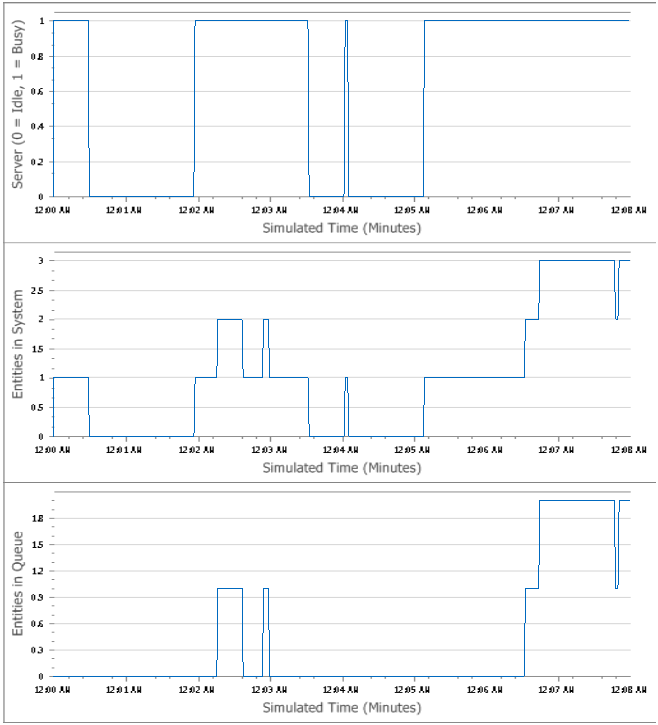
Figure 3.10: Plots of the \(B(t)\), \(L(t)\), and \(L_q(t)\) curves for the manual simulation.
In rows 36-38 we compute the output performance measures, using the built-in Excel functions =AVERAGE, =MIN, =MAX, and =SUM (have a look at the formulas in those cells). Note that the time averages in O36..Q36 are computed by summing the individual rectangle areas and then dividing by the final simulation clock time, 8, which is in A35. As examples of the final output performance measures, the server was busy 62.32% of the time (O36), the average time in system and in queue were respectively 0.8676 minute and 0.2401 minute (M36 and N36), and the time-average length of the queue is 0.3864 entities (Q36). In Chapter 4 we’ll do this same model in Simio (the actual source of the “given” input interarrival and service times) and we’ll confirm that we get all these same output performance measures.
If you’re alert (or even awake after the numbing narrative above), you might wonder why we didn’t compute standard deviations, perhaps using Excel’s =STDEV function, for the observations of times in system and times in queue in columns M and N, to go along with their means, minima, and maxima as we did in Model_03_03.xls for the monthly profits (doing so for the entries in columns O-Q wouldn’t make sense since they need to be weighted by time-durations). After all, we’ve mentioned output variation, and you can see from just looking at columns M and N that there’s variation in these times in system and times in queue. Actually, there’s nothing stopping us (or you) from adding a row to compute the standard deviations, but this would be an example of doing something just because you can, without thinking about whether it’s right (like making gratuitously fancy three-dimensional bar charts of simple two-dimensional data, which only obfuscates). So what’s the problem with computing standard deviations here? While you’ve probably forgotten it from your basic statistics class, the sample variance (of which the standard deviation is just the square root) is an unbiased estimator of the population variance only if the individual observations are statistically independent of each other — there comes a time in the proof of that fact where you must factor the expected value of the product of two observations into the product of their individual expectations, and that step requires independence. Our times in system (and in queue) are, however, correlated with each other, likely positively correlated, since they represent entities in sequence that simply physically depend on each other (so this kind of within-sequence correlation is called autocorrelation or sometimes serial correlation). If this is a single-teller bank and you’re unlucky enough to be right behind (or even several customers behind) some guy with a bucket of loose coins to deposit, that guy is going to have a long time in system, and so are you since you have to wait for him! This is precisely a story of positive correlation. So a sample standard deviation, while it could be easily computed, would tend to underestimate the actual population standard deviation in comparison to what you’d get from independent samples, i.e., your sample standard deviation would be biased low (maybe severely) and thus understate the true variability in your results. The problem is that your observations are kind of tied to each other, not tied exactly together with a rigid steel beam, but maybe with rubber bands, so they’re not free to vary as much from each other as they would be if you cut the rubber bands and made them independent; the stronger the correlation (so the thicker the rubber bands), the more severe the downward bias in the sample-variance estimator. This could lull you into believing that you have more precise results than you really do — a dangerous place to be, especially since you wouldn’t know you’re there. And for this same reason (autocorrelation), we’ve also refrained from making histograms of the times in system and in queue (as we did with the independent and identically distributed monthly profits in Model_03_03.xls), since the observed times’ being positively autocorrelated creates a risk that the histogram would be uncharacteristically shifted left or right unless you knew that your run was long enough to have “sampled” appropriately from all parts of the distribution.
One more practical comment about how we did things in our spreadsheet: In columns M-Q we computed and saved, in each event row, the individual values of observed times in system and in queue, and the individual areas of rectangles under the \(B(t)\), \(L(t)\), and \(L_q(t)\) curves between each pair of successive events. This is fine in this little example, since it allowed us to use the built-in Excel functions in rows 36-38 to get the summary output performance measures, which was easy. Computationally, though, this could be quite inefficient in a long simulation (thousands of event rows instead of our 17), or one that’s replicated many times, since we’d have to store and later recall all these individual values to get the output summary measures. What actually happens instead in simulation software (or if you used a general-purpose programming language rather than a spreadsheet), is that statistical accumulator variables are set up, into which we just add each value as it’s observed, so we don’t have to store and later recall each individual value. We also would put in logic to keep a running value of the current maximum and minimum of each output, and just compare each new observation to the current extreme values so far to see if this new observation is a new extreme. You can see how this would be far more efficient computationally, and in terms of storage use.
Finally, the spreadsheet Model_03_05.xls in Figure 3.9 isn’t general, i.e., it won’t necessarily remain valid if we change the blue-shaded input arrival times and service times, because the formulae in many cells (the pink-shaded ones) are valid only for that type of event, and in that situation (e.g., a departure event’s logic depends on whether the queue is empty). Spreadsheets are poorly suited for carrying out dynamic discrete-change simulations, which is why they are seldom used for this in real settings; our use of a spreadsheet here is just to hold the data and do the arithmetic, not for building any kind of robust or flexible model. In Section 3.4.1 we’ll briefly discuss using general-purpose programming languages for dynamic discrete-change simulation, but really, software like Simio is needed for models of any complexity, which is what’s covered in most of the rest of this book.
3.3.2 Model 3-6: Single-Server Queueing Delays
Spreadsheets are everywhere, and everybody knows at least a little about them, so you might wonder about building complete, general, and flexible dynamic simulation models inside spreadsheets. We used spreadsheets for the static stochastic Monte Carlo simulations in Section 3.2, but they could have been done more efficiently in a programming language. In Section 3.3.1 we used a spreadsheet to hold our numbers and do our arithmetic in a manual dynamic simulation, but because the formulas in that spreadsheet depended on the particular input data (interarrival and service times), it was not at all like a real model of any completeness, generality, or flexibility. While it’s difficult, if not practically impossible, to use a spreadsheet to do anything but the very simplest of dynamic simulations in a general way, spreadsheets have been used extensively for static simulations like those in Section 3.2 (see Section 3.1.1 for the difference between static and dynamic simulation).
While the single-period inventory problem in Section 3.2.3 discussed the passage of time (the first month was the peak period, and the time thereafter was the clearance-price period), time did not play an explicit role in the model. You could just as easily think of the peak period as a single instant, followed immediately by a single clearance-price instant. So that really was a static model in terms of the role played by the passage of time (it played no role). In this section we’ll simulate a very simple dynamic single-server queueing model in a spreadsheet model where the passage of time plays a central role in the operation of the model. However, being able to do this within the confines of a spreadsheet depends heavily on the fact that there happens to be a simple recurrence relation for this one special case that enables us to simulate the output process we want: the waiting times in queue (excluding their service time) of entities. Unlike the manual simulation in Section 3.3.1, we won’t be able to compute directly any of the other outputs here.
For a single-server queue starting empty and idle at time 0, and with the first entity arrival at time 0, let \(A_i\) be the interarrival time between entity \(i-1\) and entity \(i\) (for \(i = 2, 3, ...\)). Further, let \(S_i\) be the service-time requirement of entity \(i\) (for \(i = 1, 2, ...\)). Note that the \(A_i\)’s and \(S_i\)’s will generally be random variables from some interarrival-time and service-time probability distributions; unlike in Chapter 2, though, these distributions could really be anything since now we’re simulating rather than trying to derive analytical solutions. Our output process of interest is the waiting time (or delay) in queue \(W_{q,i}\) of the \(i\)th entity to arrive; this waiting time does not include the time spent in service, but just the (wasted) time waiting in line. Clearly, the waiting time in queue of the first entity is 0, as that lucky entity arrives (at time 0) to find the system empty of other entities, and the server idle, so we know that \(W_{q,1} = 0\) for sure. We don’t know, however, what the subsequent waiting times in queue \(W_{q,2}, W_{q,3}, ...\) will be, since they depend on what the \(A_i\)’s and \(S_i\)’s will happen to be. In this case, though, once the interarrival and service times are observed from their distributions, there is a relationship between subsequent \(W_{q,i}\)’s, known as Lindley’s recurrence (Lindley 1952): \[\begin{equation} W_{q,i} = \max(W_{q,i-1} + S_{i-1} - A_i, 0), \mbox{ for } i = 2, 3, \ldots, \tag{3.6} \end{equation}\] and this is anchored by \(W_{q,1} = 0\). So we could “program” this into a spreadsheet, with a row for each entity, once we have a way of generating observations from the interarrival and service-time distributions.
Let’s assume that both of these distributions are exponential, with mean interarrival time 1.25 minutes, and mean service time 1 minute; we’ll also assume that all observations within and across these distributions are independent of each other. So we next need a way to generate observations from an exponential distribution with given mean, say, \(\beta > 0\). It turns out (as will be discussed in Section 6.4) that a general way to do this (or at least try to do this) for continuous distributions is to set \(U = F(X)\), where \(U\) is a random number distributed continuously and uniformly between 0 and 1, and \(F\) is the cumulative distribution function of the random variable \(X\) desired. Then, try to solve this for \(X\) to get a formula for generating an observation on \(X\), given a generated random number \(U\). In the case of the exponential distribution with mean \(\beta\), the cumulative distribution function is \[\begin{equation} F(x) = \left\{ \begin{array}{l l} 1 - e^{-x/\beta} & \quad \mbox{if $x \ge 0$}\\ 0 & \quad \mbox{otherwise}\\ \end{array} \right.. \tag{3.7} \end{equation}\] Setting \(U=F(X)\) and solving for \(X\) yields, after a few lines of algebra, \[\begin{equation} X = -\beta\ln(1-U) \tag{3.8} \end{equation}\] where \(\ln\) is the natural (base \(e\)) logarithm function.
So, armed with Lindley’s recurrence in (3.6) and a formula for generating observations from an exponential distribution, in (3.8) plus of course our handy (if crude) Excel random-number generator RAND(), we’re ready to simulate in Excel the waiting-time process (for a little while, anyway) from a single-server queue with exponential interarrival and service times.
Figure 3.11 shows the file Model_03_06.xls, with rows 26-101 hidden to save space (open that file to see all the rows, and most importantly, the formulas in the cells). The blue-shaded cells A4..B6 contain the model’s input parameters, and the traffic intensity \(\rho\) and steady-state expected waiting time in queue \(W_q\) are computed from them in A8..B9 (see Chapter 2 for these formulas for this \(M/M/1\) queue). The entity numbers \(i = 1, 2, ..., 100\) are in column D (we arbitrarily decided to “run” this for 100 entities’ waiting times in queue), so each of these rows represents an entity finishing its waiting time in queue. Column E generates the interarrival times \(A_i\) via the Excel formula \(=-\$B\$5*LN(1 - RAND())\) where cell B5 contains the mean interarrival time; column F similarly generates the service times (LN is the built-in Excel function for the natural logarithm). Column G then implements Lindley’s recurrence from ((3.6)); for example, cell G20 (for entity \(i = 17\)) contains the formula \(=MAX(G19 + F19 - E20, 0)\) for \(W_{q,17}\) from \(W_{q,16}\) in cell G19, \(S_{16}\) in cell F19, and \(A_{17}\) in cell E20. Note that we do not have the __$__s on these cell references since we want their rows to change as we copy these formulas down; this indicates the dependence (autocorrelation) between the waiting times in queue, a behavior that will be important to developing proper statistical-analysis methods for simulation output (we can’t treat successive observations in simulation output as being independent, unlike traditional classical statistical analysis, as discussed near the end of Section 3.3.1).
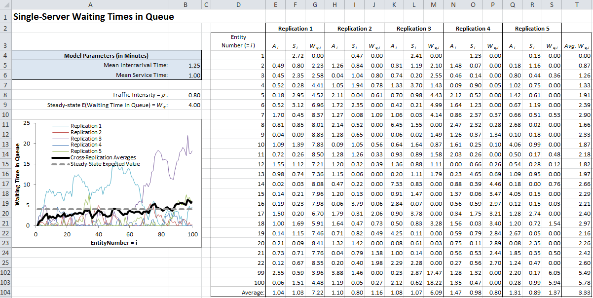
Figure 3.11: Waiting times in queue in single-server queue with Excel.
Columns E-G are then simply copied across to the right four times, to get a total of five independent replications of this 100-entity waiting-time-in-queue spreadsheet simulation; these blocks of three columns each are not changing in any way, except of course that they are all using independent draws from the volatile random-number generator RAND(). Column T averages, for each \(i = 1, 2, ..., 100\), the five values of each \(W_{q,i}\) across the five replications, so this column contains a cross-replication average of the waiting times of the first, second, …, 100th arriving entities in the five replications. Row 104 contains column averages for the \(A_i\)’s and \(S_i\)’s; these merely confirm (estimate) the mean interarrival and service times in cells B5 and B6, but for the \(W_{q,i}\)’s they are within-replication averages of the waiting times for each of the five replications separately. (We refrain from computing standard deviations of the waiting times within the replications, and we likewise don’t show histograms of these within-replication waiting times, due to the biasing effect of the autocorrelation, as discussed in Section 3.3.1.) The plot on the left shows the waiting times for each replication (light wiggly lines) as a function of the entity number, the cross-replication waiting-time-average process (heavy wiggly line, but not as wiggly as the light lines), and the steady-state expected waiting time in queue (non-wiggly horizontal dashed line).
Tap the F9 key a few times to exercise the volatility of RAND(), and watch all the interarrival, service, and waiting times change, and watch the wiggly lines in the plot jump around (the vertical axis on the plot auto-scales in response to the maximum waiting time with each tap of F9 and re-generation of all the random numbers). Notice:
- All the simulation-based curves are “anchored” on the left at 0, merely confirming that the first lucky entity to arrive has a zero wait in queue every time. But generally, as time goes by (as measured by the entity number on the horizontal axis, at least ordinally), the waiting times tend to creep up, though certainly not smoothly or monotonically due to the random noise in the interarrival and service times.
- The heavy wiggly line doesn’t wiggle as much as the light wiggly lines do, since it’s the average of those light lines, and the large and small values for each entity number tend to dampen each other out.
- All the wiggly lines, both light and heavy, have a “meandering” character to them. That is, they’re certainly random, but as you follow each line to the right, the new values are tied, at least loosely, to those that came not too long before them. This confirms the (positive) autocorrelation of the waiting times within a replication, as you can see algebraically from Lindley’s recurrence in (3.6), and as discussed near the end of Section 3.3.1.
- While some taps of F9 might give you a reasonable convergence of the waiting times to the steady-state expected value (horizontal dashed line), most don’t, indicating that (a) there’s a lot of noise in this system, and (b) it could take a lot longer than 100 entities to “approach” long-run steady-state conditions.
Go ahead and play around with the mean interarrival and mean service times in B5 and B6, but make sure that the mean interarrival time is always more than the mean service time, or else the formula in B9 for the steady-state expected waiting time in queue \(W_q\) will be invalid (though the simulation will still be valid). See how things change, especially as the mean interarrival and mean service times get close to each other (so the traffic intensity \(\rho\) in B8 creeps upward toward 1, and \(W_q\) just keeps getting bigger and bigger).
We want to emphasize that being able to do this particular dynamic simulation in a spreadsheet depends completely on the availability of Lindley’s recurrence in (3.6); and note as well that this is just for the waiting-time-in-queue output process, and not for anything else we might like to get out of even this simple system (like queue length or server utilization, as we did in the manual simulation in Section 3.3.1). In general, for complex dynamic systems we’ll have nothing like Lindley’s recurrence available, so simulating realistic dynamic systems in a spreadsheet is completely impractical, and almost always outright impossible. That’s why you need special dynamic-simulation software like Simio.
3.4 Software Options for Dynamic Simulation
In Section 3.3 we struggled through two different approaches (manual and in a spreadsheet) for carrying out dynamic simulations, neither of which is at all acceptable for anything serious. In this section we generally describe two more realistic ways to approach execution of dynamic simulations.
3.4.1 General-Purpose Programming Languages
The manual-simulation logic described and painstakingly carried out in Section 3.3.1 can be much more efficiently and generally expressed in a general-purpose procedural programming language like C++, Java, or Matlab, rather than in a spreadsheet. Historically, this is how all simulations were done before the advent of special-purpose simulation software. It’s still done today in some situations, where the model is at least relatively simple or there is need for great computer speed. However, it’s still quite painstaking (though not as bad as manual simulation with a spreadsheet as in Section 3.3.1), slow to develop, and error-prone; it does have the advantage, though, of affording almost complete flexibility to model even the quirkiest of behaviors that can’t be envisioned by developers of high-level special-purpose simulation software.
When using a general-purpose programming language for a dynamic discrete-change simulation, you still need to identify the events, and define the logic for each of them. Then, you write a subprogram (or function) to carry out the action for each type of event (actually, even the indenting of the multi-level bullet points in Section 3.3.1 for the general logic of the Arrival and Departure events suggests how these subprograms might be structured). The event subprograms are tied together with some sort of main program or function that determines the next event and directs execution to the corresponding event subprogram, and takes care of everything else we did in the manual simulation of Section 3.3.1, like event-calendar updating. At the end, you need to program the appropriate statistical summarization and create the output. You also need to be concerned with random-number generators (for stochastic simulations), how to generate observations from the desired input probability distributions, and keep track of the model state variables in some sort of data structure. As you’re seeing, this will be quite a lot of work for models of much complexity, so it can take a lot of analyst time, and is prone to errors, some of which can be very hard to detect.
Nonetheless, people still do this sometimes, perhaps as quirky modules of larger, more standard simulations. For more on this kind of programming see, for example, (Banks et al. 2005), (Law 2015), or (Seila, Ceric, and Tadikamalla 2003).
3.4.2 Special-Purpose Simulation Software
In this chapter you’ve seen various approaches to carrying out different kinds of simulations. This has included “manual” simulation, aided by a spreadsheet to keep track of things and do the arithmetic, indication of how general-purpose programming languages might be used to program a simulation along the lines of the logic in the manual simulation, and finally building general simulation models within a spreadsheet, perhaps aided by simulation-specific add-ins.
You’ve also seen that all of these approaches to doing simulation have substantial drawbacks, in different ways. Manual simulation is obviously just completely impractical for any actual application. While people have used general-purpose programming languages for simulation (and to some extent still do), which has the appeals of almost complete modeling flexibility as well as usually good execution speed, programming nontrivial dynamic simulations from scratch is hardly practical for wide use, due to the analyst time required, and the high chance of making programming errors. Spreadsheets will likely continue to be widely used for static simulations, especially with an appropriate simulation add-in, but they simply cannot accommodate the logic, data-structure, or generality needs of large-scale dynamic simulations.
Actually, people realized long ago (and long before spreadsheets) that there was a real need for relatively easy-to-use, high-level software for dynamic simulation, and specifically for discrete-change stochastic dynamic simulations. Going back into the 1960s, special-purpose simulation languages like GPSS ((Schriber 1974), (Schriber 1991)), SIMSCRIPT (Kiviat, Villanueva, and Markowitz 1969), and SIMULA (Birtwistle et al. 1973) were developed, some of which were early examples of the paradigm used by Simio, though it wasn’t called that at the time. Extensions to general-purpose programming languages like FORTRAN were developed, notably GASP (Pritsker 1974). These led to more modern, self-contained simulation languages like SLAM (Pritsker 1995) and SIMAN (C. D. Pegden, Shannon, and Sadowski 1995). All of these simulation languages, though, were really just that, languages, with text-line entry and picky syntax, so were not especially user-friendly or intuitive either to use or interpret. Graphical user interfaces, often with integrated animation, were then developed, which opened the door to far more people; these software packages include Arena (Kelton, Sadowski, and Zupick 2015), AnyLogic (www.anylogic.com), ExtendSim (www.extendsim.com), Promodel (www.pmcorp.com), Flexsim (www.flexsim.com), Simul8 (www.simul8.com), and others. For more on simulation software, see (Banks et al. 2005), (Law 2015), and especially (Nance and Sargent 2002) for comprehensive reviews; for the latest (tenth) in a sequence of biennial simulation-software surveys, see (Swain 2021).
Simio is a comparatively recent product that takes advantage of the latest in software-development and modeling capabilities. Although relatively new, Simio has been developed by the same people who pioneered the development of SLAM, SIMAN and Arena, so there is quite a lot of experience behind it. It centers around intelligent objects and provides a new object-based paradigm that radically changes the way objects are built and used. Simio objects are created using simple graphical process flows that require no programming. This makes it easier to build your own modeling objects and application-focused libraries. Simio’s flexibility and extensive integration with real-time data integration also makes it especially suitable for creating the Digital Twins necessary to support Industry 4.0. Most of this book will show you how to use simulation, and specifically Simio, to solve practical problems effectively.
3.5 Problems
Extend the simulation of throwing two dice in Section 3.2.1 in each of the following ways (one at a time, not cumulatively):
- Instead of 50 throws, extend the spreadsheet to make 500 throws, and compare your results. Tap the F9 key to get a “fresh” set of random numbers and thus a fresh set of results.
- Load the dice by changing the probabilities of the faces to be something other than uniform at 1/6 for each face. Be careful to ensure that your probabilities sum to 1.
- Use @RISK (see Section 3.2.3), or another Excel add-in for static Monte Carlo spreadsheet simulation, to make 10,000 throws of the pair of fair dice, and compare your results to the true probabilities of getting the sum equal to each of \(2, 3, ..., 12\) as well as to the true expected value of 7.
In the simulation of throwing two dice in Section 3.2.1, derive (from elementary probability theory) the probability that the sum of the two dice will be each of \(2, 3, ..., 12\). Use these probabilities to find the (true) expected value and standard deviation of the sum of the two dice, and compare with the (sample) mean in cell J4; add to the spreadsheet calculation of the (sample) standard deviation of the sum of the two dice and compare with your exact analytical result for the standard deviation. Keep the number of throws at 50.
Prove rigorously, using probability theory and the definition of the expected value of a random variable, that in Section 3.2.2, \(E(Y) = \int_a^b h(x) dx\). Start by writing \(E(Y) = E[(b-a) h(X)] = (b-a) E[h(X)]\), then use the definition of the expected value of a function of a random variable, and finally remember that \(X\) is continuously uniformly distributed on \([a, b]\) so has density function \(f(x) = 1/(b - a)\) for \(a \leq x \leq b\).
Use @RISK, or another Excel add-in for static spreadsheet simulation, to extend the example in Section 3.2.2 to 10,000 values of \(X_i\), rather than just the 50 values in
Model_03_02.xlsin Figure 3.2. Compare your results to those inModel_03_02.xlsas well as to the (almost) exact numerical integral.In the Monte Carlo integration of Section 3.2.2, add to the spreadsheet calculation of the standard deviation of the 50 individual values, and use that, together with the mean already in cell H4, to compute a 95% confidence interval on the exact integral in cell I4; does your confidence interval contain, or “cover” the exact integral? How often (tap F9 repeatedly and keep track manually)? Repeat all this, but with a 90% confidence interval, and then with a 99% confidence interval.
In the manual simulation of Section 3.3.1 and the Excel file
Model_03_04.xls, speed up the service times by decreasing them all by 20%. What’s the effect on the same set of output performance measures? Discuss.Repeat Problem 6, except now slow down the service times by increasing them all by 20%. Discuss.
In the manual simulation of Section 3.3.1 and the Excel file , change the queue discipline from FIFO to (SJF), i.e., when the server becomes idle and there’s a queue, the entity with the shortest service time will enter service next. This is also called shortest-processing-time (SPT); see Section 2.1. To do this, you’ll need to ``assign’’ the (possibly-future) service time to each entity as it arrives, and then use that to change your queue discipline. What’s the effect on the same set of output performance measures? You could do this by either (a) inserting new entities into the queue so that it stays ranked in increasing order on service time (so the entity with the shortest service time will always be at the front of the queue), or (b) leaving the queue order as it is, with new arrivals always joining the end of the queue (if they can’t go right into service) regardless of their service time, and then searching through it each time the server becomes idle and is ready to choose the correct next entity from somewhere in the queue — the results should be identical, but which would be faster computationally (think of a long queue, not necessarily just this little example)?
In the inventory spreadsheet simulation of Section 3.2.3 and the Excel file
Model_03_03.xls, we decided, essentially arbitrarily, to make 50 replications (50 rows) and our estimates of mean profit just had whatever confidence-interval half-widths (row 59) they happened to have at the end, from that sample size of 50. ChangeModel_03_03.xlsto make 200 replications (four times as many), and as you’d expect, those half-widths get smaller — by what factor? Measure this as best you can from your output (which will be challenging due to the volatility of Excel’s random-number generator). Look up in any standard statistics book the formula for confidence-interval half widths (on the mean, using the usual normal- and \(t\)-distribution approaches), and interpret your empirical results in light of that formula. About how many replications would you need to reduce these half widths (in comparison with the original 50-replication spreadsheet) by a factor of ten (i.e., your mean estimates would have one more digit of statistical precision)?In the inventory spreadsheet simulation of Section 3.2.3 and the Excel file
Model_03_03.xls, the same numerical realization of peak-period demand in column F for a given replication (row) was used for computing profit for all five of the trial values of the order amount \(h\). Instead, you could have a separate, independent column of demands for each value of \(h\) — changeModel_03_03.xlsto do it this way instead, which is just as valid. Since our real interest is in the differences in profit for different values of \(h\), is this new method better? Remember, there’s “noise” (statistical variability) associated with your average-profit estimates, and the less noise there is, the more precise will be your estimates, of both the profit values themselves for a given value of \(h\), and especially of the differences between profits across different values of \(h\).In the inventory spreadsheet simulation of Section 3.2.3 and the Excel file
Model_03_03.xls, suppose you had the choice between either hiring a really big person to do some negotiating with your supplier to get the unit wholesale cost down to $9.00 from $11.00, or hiring a slick advertising agency for some ``image’’ hype and thus be able to charge $18.95 unit retail rather than $16.95 during the peak period (assume that the clearance retail price stays at $6.95 either way). Which would be better? Are you sure? Base your comparison on what seems to be the best (most profitable) value of \(h\) from each of the two alternatives (which may or may not be the same values of \(h\)). Try to do at least some sort of statistical analysis of your results.In Problem 11, instead of asking the advertising agency to hype toward higher price, would it be better to ask them to hype toward increasing the high end of peak-period demand from 5000 to 6000? Assume that your unit wholesale cost is the original $11.00, and that your unit peak-period and clearance prices are also at their original levels of $16.95 and $6.95, respectively. Base your comparison on what seems to be the best (most profitable) value of \(h\) from each of the two alternatives (which may or may not be the same values of \(h\)).
In the inventory spreadsheet simulation of Section 3.2.3 and the Excel file
Model_03_03.xls, instead of selling hats (at a loss) left over after the peak period, you could donate them to a charity and be able to deduct your wholesale costs from your taxable corporate income; assume you’re in the 34% marginal-tax bracket. Aside from the certain good feelings of helping out the charity, would this help out your bottom line? Base your comparison on what seems to be the best (most profitable) value of \(h\) from each of the two alternatives (which may or may not be the same values of \(h\)).The original version of Model 3-4 in Section 3.2.4 used the following distributions for the input random variables: \(Q \sim \textrm{Uniform}(8000, 12000)\); \(P \sim \textrm{Normal(10 ,3)}\), truncated on the left at 2.0; and \(V \sim \textrm{Normal(7 ,2)}\), truncated on the left at 3.5 and on the right at 10.0. The truncations provide bounds on the values for \(P\) and \(V\). Develop a a model using these original distributions and replicate the analysis from Section 3.2.4 with this new model.
In the queueing spreadsheet simulation of Section 3.3.2 and the Excel file
Model_03_06.xls, “run” the model out to 1000 customers’ waiting times in queue, rather than just 100. Compare your results with the steady-state expected waiting time in queue \(W_q\), as opposed to those from the shorter 100-customer run. Explain.In the queueing spreadsheet simulation of Section 3.3.2 and the Excel file
Model_03_06.xls(with a “run” length of 100, as originally done), push the arrival rate up by decreasing the mean interarrival time from 1.25 minutes to 1.1 minutes and compare your results with the original model. Then, push the arrival rate up more by decreasing the mean interarrival time more, down to 1.05, then 1.01, and see how this affects your results, both the steady-state expected waiting time in queue \(W_q\), and your simulation results.Continue right on over the brink with Problem 16, and go ahead and reduce the mean interarrival time on down to 1.00, then 0.99, then 0.95, then 0.88, and finally 0.80 (be brave!). What’s happening? In light of the “stability” discussions in Chapter 2, are your results even “meaningful” (whatever that means in this context)? You might want to consider this “meaningfulness” question separately for the steady-state expected waiting time in queue \(W_q\), and for your 100-customer simulation results.
Walther has a roadside produce stand where he sells oats, peas, beans, and barley. He buys these products at per-pound wholesale prices of, respectively, $1.05, $3.17, $1.99, and $0.95; he sells them at per-pound retail prices of, respectively, $1.29, $3.76, $2.23, and $1.65. Each day the amount demanded (in pounds) could be as little as zero for each product, and as much as 10, 8, 14, and 11 for oats, peas, beans, and barley, respectively; he sells only whole-pound amounts, no partial pounds. Assume a discrete uniform distribution for daily demand for each product over its range; assume as well that Walther always has enough inventory to satisfy all demand. The summer selling season is 90 days, and demand each day is independent of demand on other days. Create a spreadsheet simulation that will, for each day as well as for the whole season, simulate Walther’s total cost, total revenue, and total profit.
A new car has a sticker price (the full retail asking price) of $22,000. However, there are several customer-chosen options (automatic transmission, upgraded speakers, fog lights, auto-dimming rear-view mirror, moonroof) that can add between $0 and $2000 to the selling price of the car depending on which options the customer chooses; assume that the total cost of all options is distributed uniformly and continuously on that range. Also, many buyers bargain down the price of the car; assume that this bargain-down amount is distributed uniformly and continuously between $0 and $3000, and is independent of the options. The selling price of the car is $22,000 plus the total of the options cost, minus the bargain-down amount.
Create an Excel spreadsheet simulation that will compute the actual selling price for the next 100 cars sold, using only the capabilities that come built-in with Excel, i.e., don’t use @RISK or any other third-party add-ins. Find the sample mean, standard deviation, minimum, and maximum of your 100 selling prices. Form a 95% confidence interval for the expected selling price of infinitely many future sales (not just the next 100), and do this within Excel (: check out the built-in Excel function and be careful to understand its input parameters). Also, create a histogram of your 100 selling prices, either by mimicking what was done in Model 3-5, or by using the Data Analysis ToolPak that comes with Excel (you may need to install it via File \(>\) Options \(>\) Add-Ins, then in the Manage window at the bottom select Excel Add-ins, then the Go button just to the right, then check the box for Analysis ToolPak, then OK) and its Histogram capability (you may want to explore Excel help for this). Do everything within Excel, i.e., no side hand/calculator calculations or printed statistical tables, etc.
In a second sheet (tab) of your same Excel file, repeat part a) above, except now use @RISK or another Excel add-in for static spreadsheet simulation, including its built-in variate-generation functions rather than your own formulas to generate the uniform random variates needed; also, don’t compute the confidence interval on expected selling price. Instead of 100 cars, do 10,000 cars to get both a better estimate of the expected selling price, and a smoother histogram (use the histograms that come with @RISK). Again, do everything within Excel (other than using @RISK).
To put a finer point on Problem 19, the prices of the five available individual options and the percent of customers who choose each option are in Table 3.1 (e.g., there’s a probability of 0.6 that a given customer will choose the automatic transmission, etc.). Assume that customers choose each option independently of whether they choose any other option. Repeat first part of Problem 19, but now with this pricing structure, where each customer either will or won’t choose each option; the bargain-down behavior here is the same as in Problem 19, and is independent of customer choice of options. Do this within Excel, i.e., do not use @RISK. Hint 1: The probability that a continuous random number on [0, 1] is less that 0.6 is 0.6. Hint 2: The built-in Excel function
=IF(condition, x, y)evaluates to x if the condition is true, and to y if the condition is false.
| Option | Price | % Customers choosing option |
|---|---|---|
| Automatic transmission | $1000 | 60 |
| Upgraded speakers | $120 | 10 |
| Fog lights | $200 | 30 |
| Auto-dimming rear-view mirror | $180 | 20 |
| Moonroof | $500 | 40 |
References
The original link was http://www.geocities.com/WallStreet/9245/vba12.htm. This link appears to no longer be active, but we include it here for completeness of the citation.↩︎