Simio and Simulation: Modeling, Analysis, Applications - 7th Edition
Chapter 10 Miscellaneous Modeling Topics
The goal of this chapter is to discuss several modeling concepts and related Simio features that will enhance your modeling skills. The sections in this chapter will generally stand on their own — there is no “central theme” that should be followed from beginning to end and you can pick and choose the sections to cover and the sequence based on your modeling needs.
10.1 Search Step
The Search step is a very flexible process step that is used to search for objects and table rows from a collection in a model. A collection is a group of objects in a model. Examples of collection types include Entity Populations, Queue States, Table Rows, Object Lists, Transporter Lists, and Node Lists (see the Help for a complete list of collection types). In this section, we describe two example models that demonstrate the use of the Search step. Several additional Search-related examples are available in the SimBit collection (from Simio, choose the Support ribbon and click on the Sample SimBit Solutions item and search the collection using the Search keyword).
10.1.1 Model 10-1: Searching For and Removing Entities from a Station
In this model, we want arriving entities to wait in a “holding station” from which they are periodically pulled and processed. This effectively decouples the entity arrival process from the entity processing. Figure 10.1 shows the completed model.
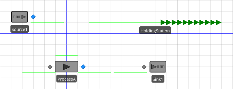
Figure 10.1: Model 10-1.
The queue state labeled Holding Station is associated with a Station Element defined in the model (see Figure 10.2).
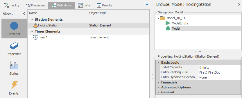
Figure 10.2: Definitions for Model 10-1.
The queue in the Facility View is placed using the Detached Queue button from the Animation ribbon (the queue state name is HoldingStation.Contents). Entities are transferred from the Source1 object to the station using the CreatedEntity add-on process trigger (see Figure 10.3).
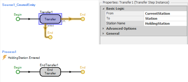
Figure 10.3: The two processes associated with transferring entities from Source1 to HoldingStation.
Process1 uses the End Transfer step to finalize the transfer of the entity. Note that this process is triggered by the event HoldingStation.Entered which is automatically fired when an entity enters the station.
With the logic described so far, created entities would be transferred directly to the holding station where they would remain indefinitely (until the end of the simulation run). Since we want to periodically pull the entities out of the holding station and process them, we will use a process triggered by a timer to search the holding queue and transfer any entities to the input node of ProcessA for processing. Figure 10.4 shows this process (PullEntities). In the Search step, we set the Collection Type to QueueState, the Queue State Name to HoldingStation.Contents, and the Limit to Infinity. With these property settings, the Search step will search the HoldingStation queue for all entities. Each found entity is then transferred to the input node of the ProcessA object. Note also that the process is triggered by the timer event (Timer1.Event – see Figure 10.2 for the timer definition). While this simple example uses a timer to periodically pull entities from the station, the same search logic could be used with many other pull or push mechanisms.
We recommend that you experiment with this model by changing the arrival process (Source1) and/or the timer intervals (Time1) and observe the impact on the model. You should also run this model with Trace on so that you can see the precise sequence of model events as the model runs.
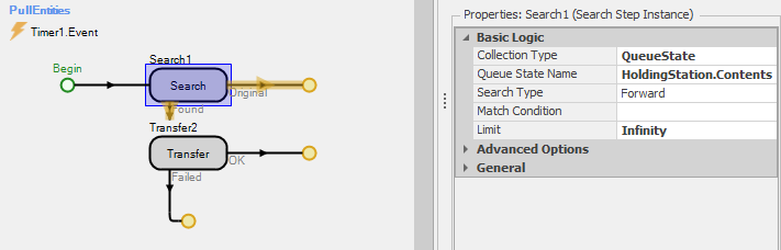
Figure 10.4: Process for searching the holding queue and transferring the entities to ProcessA.
10.1.2 Model 10-2: Accumulating a Total Process Time in a Batch
In this second example of using the Search step, we want to batch entities and determine the processing time for the batch by summing the individual processing times for the entities comprising the batch. Figure 10.5 shows the completed model. Source1 creates type A entities (the Parent entities for the batches) and Source2 creates type B entities (the Member entities for the batches). The user-defined entity state ProcessTime is used to store the individual process times for type B entities and the total processing time for the batch (the type A entities) — the accumulated value. As shown in Figure 10.5, processing time values are randomly assigned to type B entities using a triangular distribution with parameters (1, 2, 3). We used an exponential distribution with mean of 1 minute for the Source1 interarrival time and we also animated the BatchMembers queue for Entity instance A in order to visualize the batches.
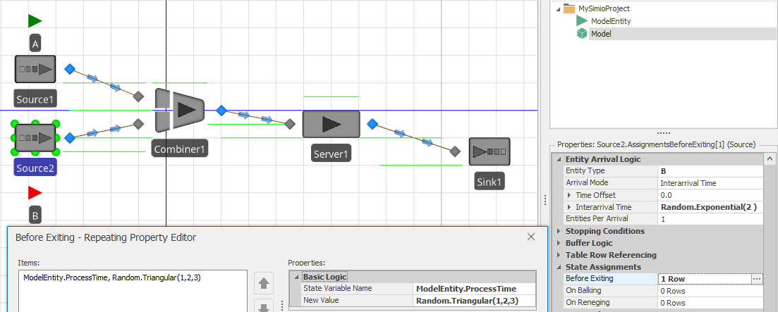
Figure 10.5: Definitions for Model 10-2.
The combiner (Combiner1) object batches one type A entity with five type B entities. Hence, we would like for the processing time for the batch at Server1 to be the sum of the five values assigned to the type B entities prior to batching. We use the Processing add-on process trigger with Combiner1 so that the batch will be formed before the associated process is executed. Figure 10.6 shows the process. Here we use the Search step to find all entities in the batch queue (ModelEntity.BatchMembers) and sum the values of the expression specified in the Search Expression property (Candidate.ModelEntity.ProcessTime). This will sum the values of the specified expression and store the sum in the token return value. We can then assign this sum (Token.ReturnValue) to the ProcessTime state of the batch in the subsequent Assign step and use this state for the Processing Time property in Server1. As a result, the individual batch components of type B will each have a sampled process time and the batch will have the sum of these times as its process time.
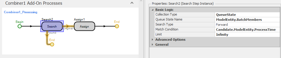
Figure 10.6: Add-on process for summing the process times in Model 10-2.
Before we leave discussion of the Search step, a warning is in order. The Search step is very powerful and can do many things, but there is a downside - the potential for overuse. Say, for example, that you have a table of 10,000 rows or a collection of 10,000 entities that you perhaps want to search at every time advance to determine the next appropriate action. While Simio can do this for you easily, you might notice that your execution speed becomes noticeably slower. Overuse of searches is a common cause of execution speed problems.
10.2 Model 10-3: Balking and Reneging
Balking and reneging are common queueing behaviors that can be tricky to model. Balking occurs when an arriving entity chooses not to enter a queue (e.g., a potential customer deciding that a line is too long and bypassing the system). Reneging occurs when an entity in a queue chooses to leave before receiving service (e.g., you wait in line for a little while and decide that the line is moving too slowly and you leave). Jockeying or line-switching is a related queue behavior which occurs when a customer reneges from one line and joins another. Fortunately, Simio offers comprehensive support for both balking and reneging using the Buffer Logic properties in objects from the Standard Library. Model 10-3 is a modified version of the ATM model from Section 4.4 where we incorporate basic balking and reneging behaviors for the ATM customers. In the modified model, arriving customers should balk if there are already 4 customers waiting in line and customers already in line should probabilistically leave the line once they’ve been in line for 3 minutes (we chose these two values arbitrarily – the actual values that you would use would be situation-specific).
Figure 10.7 shows Model 10-3 with the ATM1 object properties displayed. We have added two additional sink objects – balking entities will be sent to the Balks sink and reneging entities will be sent to the Renegs sink (in our model, we also added Status Labels that display the number of entities that enter each Sink to improve the visibility). Note in the properties window that the Input Buffer Capacity for the ATM1 object is set to 4 and the Balk Decision Type property is set to Blocked. This indicates that when an entity arrives to a full buffer, that rather than blocking on the network (the default behavior), the arriving entity will be transferred to Input@Balks.
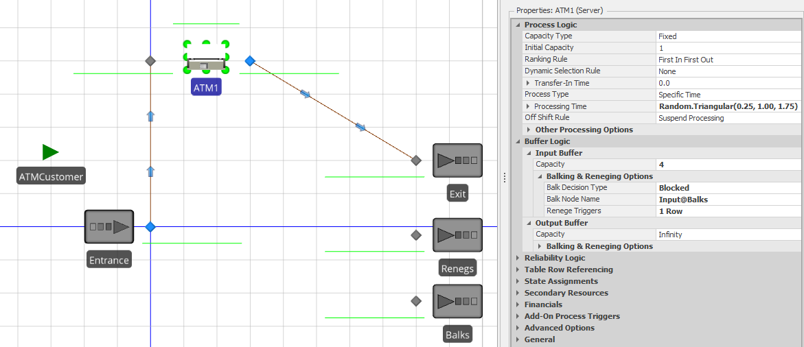
Figure 10.7: Model 10-3 and the ATM1 object properties.
The reneging behavior is specified by the Renege Triggers property group (see Figure 10.8. Here we specify that after waiting for 3 minutes, the entity should renege with probability 0.5. Those entities that do renege are sent to Input@Reneges (the input node to the sink). The entities that “fail” the probability test will simply remain in the queue.
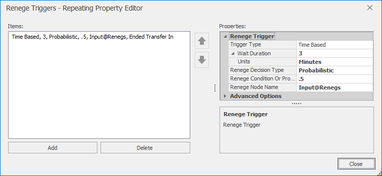
Figure 10.8: Renege Triggers properties for Model 10-3.
While the balking and reneging behaviors in Model 10-3 are quite basic, similar methods can be used to develop quite complex (and comprehensive) balking, reneging, and jockeying behavior in models. As with most other Simio-specific topics, there are several SimBit Solutions that demonstrate the use of balking and reneging, including:
BalkingOnSourceBlockingOnServer - Simple balking on a source with no buffer space.
ChangingQueuesWhenServerFails - Entities waiting at one server change to another server when their server fails.
ServerQueueWithBalkingAndReneging - Entities have individual number in line tolerances which causes balking as well as individual waiting time tolerances which cause them to renege IF they are not close (within their personal stay zone) to being served.
MultiServerSystemWithJockeying - Whenever another line becomes shorter than the one entity is waiting in, it will move (jockey) to a shorter line.
10.3 Material and Inventory Elements
This section introduces the Material and Inventory elements. These elements are extremely useful for supply chain-type applications where you consume material at one location and produce material at another location and/or need to represent items using a Bill of Materials structure. Note that these elements have many features and options and our goal here is simply to introduce them and provide some SimBit references to demonstrate their use, not to provide a comprehensive guide to their use.
Material Elements are used where you need to keep track of a quantity of things (like raw materials, finished goods, sub-assemblies, etc.), but you do not need the features associated with Entity populations. With a Material Element, you define an initial quantity in stock when the model starts and during the run, you can produce the material (increasing the quantity in stock) and consume the material (decreasing the quantity in stock). The material production and consumption operations can be done in Simio Processes using the Produce and Consume steps, respectively, and also as part of Task Sequences (see 10.4). Some important features of the Material element are:
Assume Infinite - If a Material element’s Assume Infinite property is set to
False, the process execution (for a Consume step) or task execution (for a Task Sequence) will be blocked if the Material’s quantity in stock is less than the consume amount and will remain blocked until the requested quantity is made available through a Produce step or task. If the property is set toTruethe Material’s quantity in stock will be allowed to go negative (and no blocking will occur).BOMs - A Material can represent a single material or a Bill of Materials comprised of other materials in user-specified quantities. This feature is especially useful – when a BOM Material is consumed, the individual Materials comprising the BOM are consumed automatically. In a product assembly context, for example, the component materials for the assembly are consumed with a single Consume step/task during the assembly operation and the assembled product is produced using Produce step/task.
Replenishment - Materials elements support several standard replenishment policies where the material is automatically replenished based on the policy (such as min/max, reorder point/reorder quantity, and order up-to). These policies give the model developer tremendous flexibility in how the policies are implemented.
Location-based - A Material can be “global” to the model or attached to any object in the model (a Server object or Node object, for example) using an Inventory element (see below). Location-based Materials simplify the implementation of models where materials are moved from one model location to another, like from a supplier to a warehouse to a manufacturing facility to a retail outlet, for example.
An Inventory Element defines a “bucket” that holds a specific Material and is attached to a model object. So, if a Material is not location-based, you can think of producing to and consuming from a “global bucket” of that Material, whereas if the Material is location-based, you produce to and consume from specific Inventories of that Material. In the supply chain example above, a model might have one Inventory element associated with an object representing a supplier, another Inventory element associated with an object representing a warehouse, and a third Inventory element associated with a manufacturing facility. To “move” material through the supply chain, you would consume from the supplier Inventory element and produce to the warehouse Inventory element, consume from the warehouse Inventory element and produce to the manufacturing facility Inventory element.
We suggest reviewing the following SimBit models for more information and example uses of the Material and Inventory elements:
SimBit: Server With Material Consumption illustrates the basic use of a Material element.
SimBit: Inventory and Materials illustrates the use of Materials and corresponding site-based Inventory elements.
SimBit: Inventory Replenish illustrates inventory replenishment using several policies.
SimBit: Constraint Logic illustrates how to use the Constraint Logic element to hold an entity when a Material requirement constraint is not met.
10.4 Model 10-4: Task Sequences
Since we first introduced the Server object in Chapter 4 we have always left the Process Type property set to Specific Time. This results in a single-phase operation with a single associated processing time. What if you want something more complex like (for example) multiple operations in sequence or in parallel or execution based on conditions? Simio has a solution – Task Sequences.
Task Sequences define and execute a structured sequence of processing tasks. The easiest way to use them is to specify a Process Type of Task Sequence on a Server, which then exposes a Processing Tasks repeat group of Tasks to be executed. Note this capability is also found on the Combiner and Separator and can also be used via the Task Sequences Element directly. A Task in a Task Sequence can be as simple as a processing time, or can have many more options like secondary resources, material requirements, state assignments and add-on processes. A sequence might have a single task, or many of them. If you have multiple tasks, they can be executed sequentially, in parallel, conditionally, probabalistically, and in any combination of these options.
Let’s illustrate with a very simple scenario. Consider a two-stage painting operation where the first stage is Prepare, requiring 0.5 to 1.5 minutes (uniform) and the second stage is Paint requiring 0.5 to 2.0 minutes with a mode of 1.0 minutes (triangular). Parts arrive to the system according to an exponential distribution with a mean interarrival time of 2.5 minutes. While this simple system could easily be modeled using two servers, since it all happens at a single location, let’s model it with a single two-stage server instead.
Add a Source, Server, and Sink, and set the source properties appropriately.
On the server we will need to specify a Process Type of
Task Sequence.Click on the
Processing Tasksto open the repeat group of Tasks.Add a task. Change the Name to
Prepare, and the Processing Time toRandom.Uniform(0.5, 1.5). Leave all other fields at their default values.Add a second task. Change the Sequence Number to
20, indicating that it must follow task “10”, the first one. Set the Name toPaint, and the Processing Time toRandom.Triangular(0.5, 1.0, 2.0). Again, leave all other fields at their default values.Your work should look similar to Figure 10.9.
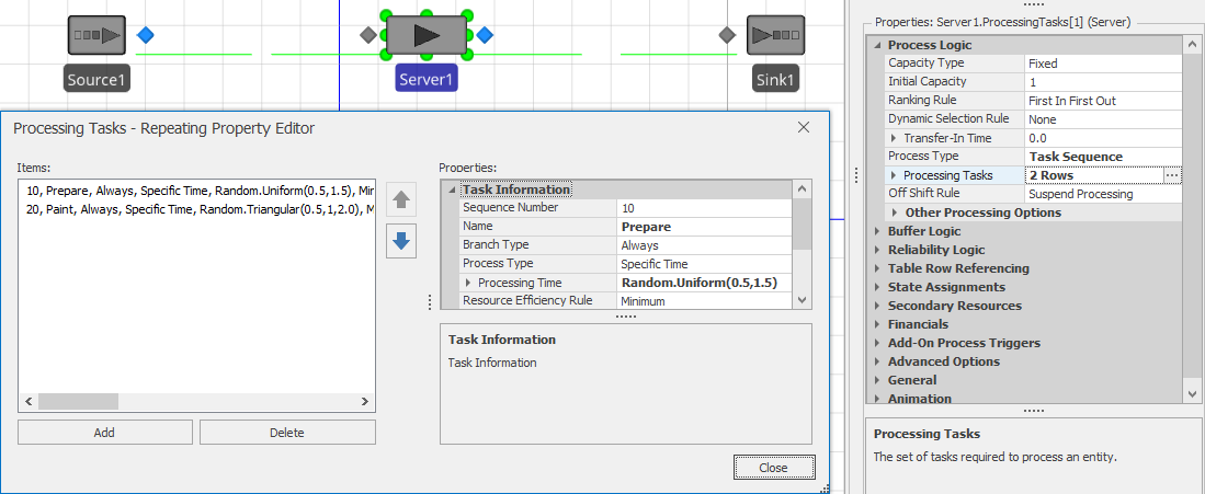
Figure 10.9: Task Sequences repeat group for Model 10-4 (Initial).
If you run the model now it should appear to work, but it is difficult to tell if it is working correctly. We encourage you to examine the operation in the Trace window using Step to study the behavior of a single entity moving through the system.
Let’s make an enhancement to the model that will allow us to learn more features and illustrate more clearly that the model is working. Let’s assume that this model has a worker named Prepper, with home node BasicNode1 placed in the vicinity of the source. And the model has a second worker named Painter with home node BasicNode2, placed in the vicinity of the sink. Both workers should return to their home location when idle. We also have a third BasicNode named WorkPlace that is placed just above the place where the entity waits while processing on the server.
If you go to the server and reopen the Task Sequences repeat group, you will note a Resource Requirements section that is similar to the previously resource specifications. Change both tasks (the first is illustrated in Figure 10.10 so that you request the appropriate worker and have him come to the WorkPlace node to do the work. Now when you run the model, you should see the Prepper approach from the left to do the Prepare task and then immediately see the Painter approach from the right to do the Paint task.
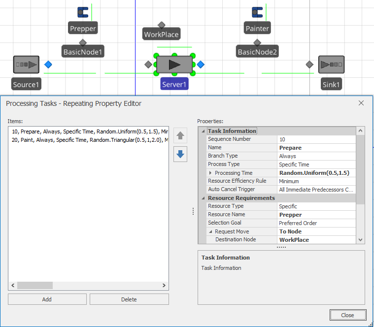
Figure 10.10: Task Sequences repeat group for Model 10-4 (Final).
Just as we specified resource requirements above, in that same task repeat group we can also specify Material Requirements (see in Section 10.3). Here we have the choice to either produce or consume Materials as well as to produce or consume a Bill of Materials (e.g., the list of materials required to make up another material).
Every task also has a Branch Type that helps determine under what circumstances the task should be done. In our above example, we used the default of Always, indicating, as the name implies that we will always do both of those tasks. But other choices include Conditional, Probabilistic, and Independent Probabilistic. For example, we might have specified the Probabilistic branch type on Preparation if that task only needed to be done, say 45% of the time. Note that at the beginning of this paragraph we used the phrase “helps determine” if the task should be done. Another consideration on whether a task should be done is based on if its previous task was cancelled (e.g., if Preparation isn’t needed, should I still do Paint anyway?). The Auto Cancel Trigger property defaults to cancelling the task if All Immediate Predecessors Cancelled is selected, but can also let the task proceed if you choose None for the action.
When you have more than one task, you must specify in what order to process them. In our model above, we just specified sequential task numbers (e.g., 10 and 20). For relative simple sequences, this is probably the easiest way. If you refer back to the server, you will see an Other Task Sequence Options grouping which contains a Task Precedence Method property. In addition to the Sequence Number Method which we already used, you can also choose from Immediate Successor and Immediate Predecessor. These latter two options often are much easier to use to create complex sequence diagrams like Figure 10.11.
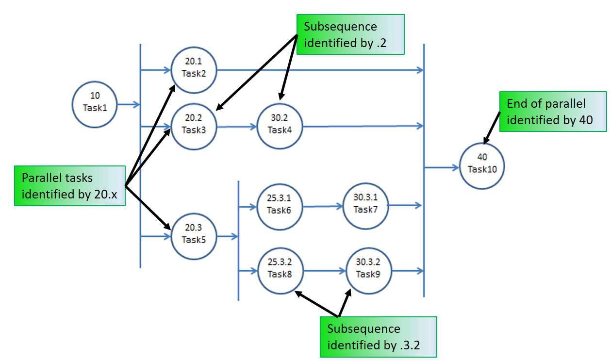
Figure 10.11: More complex task sequence using sequence numbering.
Recall that when we introduced the server, we skipped over the Process Type property and just used Specific Time, until we thought you were ready to learn about Task Sequences. Well, we’ve done it again. Each task in the sequence has a Process Type that we skipped over until now. We are still not going to cover the details here, but it is worth mentioning that a task is not limited to a simple processing time. You can also select Process Name to execute a process of any length; Submodel to send an entity clone to a submodel (e.g., a set of objects) and wait for it to complete; or Sequence Dependent Setup to automatically calculate processing time based on data specified in a Changeover Logic element.
One final note on task sequences … in some applications there are many, perhaps hundreds, of tasks completed at a single station. For example, when you are assembling an airplane, the plane might move to position one and have dozens of crews execute hundreds of tasks over several days, then the plane moves to position two for more work. Manually entering that into a task sequences like we have illustrated above would be tedious. Many such models are data driven as described in Section 7.7 The Other Task Sequence Options in the server properties contains some additional options to support data driven task sequences. We suggest reviewing the following models for more information:
SimBit: ServerUsingTaskSequenceWithWorkers illustrates four serial tasks used with workers.
SimBit: TaskSequenceAndWorker illustrates concurrent tasks that move around worker.
SimBit: ServerUsingTaskSequenceAlternativeMethodsForDefiningTaskPrecedence illustrates different task precedent definitions
SimBit: ServersUsingTaskSequenceWithDataTablesJobShop illustrates use with data tables.
Example: HealthCareClinic illustrates all task data specified in relational data tables.
10.5 Event-based Decision Logic
As we learned in Section 5.1.1.1, events are messages that can be fired to communicate between objects. Events are useful for informing other objects that something important has happened and for incorporating custom logic. Let’s look at that topic in a bit more depth.
There are many ways to generate events in Simio, in fact, many events are automatically defined and triggered. For example, every time an entity enters or exits a node, an event is generated. Since most models have nodes at the entry and exit of most objects, this gives a very easy way to detect important state changes and trigger other things to happen. Likewise a number of Standard Library objects can respond to selected events. For example, if you want to have just-in-time arrivals of pallets into a system, you can use the Arrival Mode on a Source to cause creation of objects only when a pallet leaves a specified node. Refer to the SimBit RegeneratingCombiner for an example.
There are many other automatic events that are produced by the Standard Library objects, including:
When an entity begins or ends a transfer or is destroyed.
When a resource is allocated or released, changes capacity, or is failed or repaired.
When a server changes capacity, or is failed or repaired.
When a worker or vehicle enters or leaves a node, begins or ends a transfer, is allocated or released, changes capacity, or is failed or repaired.
Likewise many Standard Library object actions are triggered by events, including:
Source can trigger entity creation (as discussed above).
Source can stop creating entities.
Server, resource, conveyor, or vehicle can start a failure.
Vehicle or worker can stop a dwell time.
With all of those combinations, you might begin to realize that you can make a lot of dynamic decisions based on using properties in the Standard Library objects and the automatic events they generate. But before we demonstrate that, let’s go one level deeper. In addition to all these automatic events, you can define your own events and trigger them in very flexible ways using elements and steps. Elements and steps trigger and respond to events in a similar fashion to the Standard Library, but you have even more flexibility and control. And we can even define our own user-defined events on the Events window of the Definitions tab. Let’s examine some ways we can trigger, or “fire” our own events:
Station element - used to define a capacity constrained location for holding entities representing discrete items. Generates Entered, Exited, and CapacityChanged events.
Timer element- fires a stream of events according to a specified IntervalType. Generates event named Event each time the timer matures. The timer can also respond to external events to trigger future timer events or reset the timer.
Monitor element - used to detect a discrete value change or threshold crossing of a specified state variable or group of state variables. Generates event named
Eventeach time the monitor detects a monitored state change.Fire step - used to fire a user-defined event.
As we discussed above, many Standard Library objects have properties that allow them to act when an event is received. But we are not limited to those predefined reactions – we can define our own reactions. The two common ways of doing this are using the Wait step inside a process or triggering the Process itself.
So far all the processes we have used have been started or triggered automatically by Simio (e.g., OnRunInitialized) or by the object they are defined in (e.g., an Add-On Process). But another very useful way of triggering the start of a process is by using the property named Triggering Event Name to subscribe to a specific event. As the name implies, when the specified event is received, this process will start and a token is created which starts executing the triggered process (note that if a Triggering Event Condition is specified, then it must evaluate to True before the process is started). The Subscribe step allows you to dynamically make the same sort of relationship – typically with a specific entity. And you can dynamically cancel that relationship using the Unsubscribe step.
Another, even finer way of reacting to an event is using the Wait step. In this case, the step is inactive (e.g., it ignores all events) until a token executes the Wait step. That token will then “wait” in the Wait step until one or more of the specified events has occurred. This is commonly used to force a token (and possibly its associated object) to wait at a certain point in the model until a condition has occurred. For example, you might have all priority 2 parts wait at a node, perhaps on a conveyor, until all the priority 1 parts, perhaps on another conveyor, have been completed. The last priority 1 part might Fire an “AllDone” event that the priority 2 parts are waiting on.
While there are many simple applications of Wait and Fire, an interesting and fairly common application is the coordination or synchronization of two entities, when either entity could arrive to the coordination point first. For example perhaps we have a patient waiting to proceed to imaging (e.g., an MRI) but he cannot proceed until his insurance paperwork is approved. But the insurance paperwork cannot continue until the patient is prepared and ready to enter the MRI. It’s easy to consider having PatientReady and PaperworkReady events where each entity waits for the other. But if you don’t know which entity will arrive first that presents the problem of prematurely firing an event, before the other entity is waiting for it. The solution is to use a state variable to indicate the presence or ready state of either object, a Decide step to check that state, and then either Fire or Wait on the other entity. We will leave this to you to explore the details in the homework problems. One final note in this section is to consider alternatives to event-based logic. While the event-based approaches are generally very efficient, sometimes you need additional flexibility.
The Scan step may be used to hold a process token at a step until a specified condition is true. When a token arrives at a Scan step, the scan condition is evaluated. If the condition is true, then the token is permitted to exit the step without delay. Otherwise, the token is held at the Scan step until the condition is detected to be true. While monitoring the value of any expression offers considerable flexibility, it comes with two caveats. The condition is only checked at time advances, so it is possible that momentary (e.g., time zero) conditions can be missed and in fact, the condition itself will not be recognized until a time advance. The second caveat is that monitoring an expression is slower than an event-based approach — in most models this will not be noticeable, but in some models it could cause a slower execution speed.
The Search step discussed earlier in this chapter can often be used as a companion to event-based logic. For example when an event of potential interest is triggered, you might search a set of candidates to determine appropriate action (if any).
10.6 Other Libraries and Resources
So far we have concentrated on just the Simio Standard Library – you might agree that there is plenty to learn on those 15 objects. But we also wanted to make you aware that there are many more possibilities to be explored - in particular the Flow Library and the Extras Library that are supplied by Simio. And going beyond that, the SI Shared Items in the User Forum has many interesting items contributed by other users and the Simio GitHub repository has code for many Open Source projects supplied by the Simio Team.
10.6.1 Flow Library
While everything in the Standard Library is primarily focused on modeling discrete entity movement, fluid and fluid-like behaviors can often be more accurately modeled using continuous or flow concepts. Typical applications include pharmaceuticals, food and beverage, mining, petrochemicals, and chemicals. In fact it is useful in any applications where you have steady or intermittent streams of materials flexibly flowing down networks of pipes (or conveyors), between mixers and tanks (or storage piles), and possibly filling and emptying of containers.
While a few other simulation products also have flow capability, Simio’s capability is comprehensive. And unlike most products, Simio’s flow and discrete modeling integrate seamlessly in a single model. You can see one indication of this by examining the physical characteristics of any entity – you will find that in addition to having a 3 dimensional physical size (e.g., a volume) discrete entities also have a density. This dual representation of an entity as either a discrete item (e.g., a barrel or a pile) or as a quantity of fluid or other mass (e.g., 100 liters of oil or 100 tons of coal) allows a discrete entity to arrive to a flow construct and start converting its volume to or from flow. It also allows assigning and tracking the attributes of entities representing material flow on a link or in a tank – for each component of a flow you can track attributes like product type, routing destination, and composition data. The Flow library includes the following objects:
FlowSource - May be used to represent an infinite source of flow of fluid or other mass of a specified entity type.
FlowSink - Destroys flow that has finished processing.
Tank - Represent a volume or weight capacity-constrained location for holding flow.
ContainerEntity - A moveable container (e.g. a barrel) for carrying flow entities representing quantities of fluids or mass.
Filler - A device to fill container entities.
Emptier - A device to empty container entities.
ItemToFlowConverter - Converts discrete items to flow entities.
FlowToItemConverter - Converts flow entities to discrete items.
FlowNode - Regulates flow into or out of another object (such as a Tank object) or at a flow control point in a network of links.
FlowConnector - A direct, zero travel distance connection from one flow node location to another.
Pipe - A connection from one flow node location to another where flow travel time and pipeline volume is of significant interest.
To learn more about the Flow Library, we refer you to the Simio Help. In particular we recommend studying the SimBit FlowConcepts which contains eight models each of which illustrates a different aspect of the library.
10.6.2 Extras Library
The Extras library is designed as a supplement providing additional commonly encountered constructs. Many of these objects are composite objects which are built-up from collections of other objects. This provides benefits in that, when necessary, you can edit the graphics, behavior, or properties of the composite objects to meet the needs of your application.
The Extras library includes the following objects:
Bay - This describes a rectangular area (e.g. floor space) over which one or more bridge cranes can move. Each bay may be divided into multiple zones to prevent bridge collisions.
Crane - This represents a bridge or overhead crane. This composite object consists of the bridge itself, the cab that travels along the bridge, the lift that controls the vertical movement, and the “crane” end effector (the hook or grabbing device). The crane has similar characteristics to a vehicle (load, unload, dwell, initial node, and idle action) plus has acceleration and speed in all directions.
Robot - This represents a jointed robot that can pick up entities at one node and drop them at another node. This composite object consists of a fixed base that can rotate, a lower arm that moves in relation to the base, an upper arm that moves relative to the lower arm, and a hand or end-effector that is attached to the end of the upper arm. The robot has similar characteristics to a vehicle (load, unload, dwell, initial node, and idle action) plus has pitch and rate of change for all rotations.
Rack - The Rack is also a composite object that is comprised of the main rack, which is a fixed object representing the rack frame, and one or more associated shelves. The number of shelves that are owned by the rack, and the capacity of each shelf (i.e. the maximum number of entities that can be stored on the shelf) are two important properties of the rack.
LiftTruck - The Lift Truck is a composite object comprised of a vehicle and an associated lift device. The Lift Truck moves its associated lift device up and down to the appropriate shelf height when placing and removing entities onto and off of a shelf. In addition to the normal vehicle properties, it has two additional properties that specify the vertical lift speed and the lift travel height.
Elevator - The Elevator is a transporter that moves up and down in the vertical direction and picks up and drops off entities at its associated Elevator Nodes.
ElevatorNode - Each Elevator Node represents a destination for a specific elevator and references its associated Elevator.
There are several SimBits that demonstrate the use of the Extras Library objects – to find them, simply open the Support Ribbon, click on Sample SimBitSolutions, and enter Extras Library in the search box. There is also an example model (EngineRepairUsingExtrasLibrary) that demonstrates the use of the library.
10.6.4 Simio GitHub
The Simio LLC GitHub Site is a place where Simio team members have posted the source code and other information for Open Source projects that users may find helpful. This can be found at https://github.com/SimioLLC. These projects are released under their respective licenses and support is not guaranteed.
This repository is organized under six topic areas:
- Automations
- Data Connectors and Transformers
- Design Add-Ins
- User Defined Steps and Elements
- Third-Party Integrations
- Misc
Figure 10.12 shows a few of the popular repositories in the Simio GitHub site.
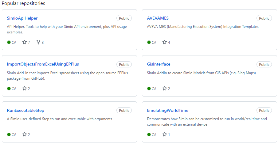
Figure 10.12: Popular repositories in the Simio GitHub site.
10.7 Experimentation
Let’s return to the topic of experimentation that we introduced in Section 4.2.3. By now, you can fully appreciate the value of running multiple replications to get a statistically valid answer and the value of running multiple scenarios in a search for the best solution. And in Chapter 9 we studied how OptQuest can help us find the best alternative from a large number of scenarios. Unfortunately one aspect these all have in common is the need to run many replications. If your replications require 1 second each and you need 100 replications, getting your results in less than 2 minutes isn’t too bad. But we recently had an application that required at least 5 replications for each of 500 scenarios for each of 9 experiments. At about 2.5 minutes per replication this called for over 900 hours of processor time. Waiting over a month for the runs to process sequentially is probably unacceptable. While this is a particularly large problem, large real projects often encounter similar situations. In this section we will discuss how to deal with such high processing demand.
10.7.1 Parallel Processing
The good news is that most modern computers feature the capability to do at least limited parallel processing and all versions of Simio take advantage of that capability. So, for example, if you have a dual-threaded quad processor, a common configuration, your hardware will support up to 8 parallel “threads” of execution, which in Simio terms means that you can run up to 8 concurrent replications. Using this feature cuts the 900 hours down to only 113 hours, but that’s still a long time to wait.
If you are lucky enough to have 16 or more processors (somewhat uncommon as of this writing) Simio will run up to 16 parallel replications on your machine. The higher editions of Simio (Professional and RPS) also support the ability to Distribute Runs to other computers in your local network (see Experiment Properties \(\rightarrow\) Advanced Options \(\rightarrow\) Distribute Runs for details). If you are fortunate enough that either of these choices is available to you, by executing up to 16 parallel replications we can now generate results in around 60 hours – still a long time, but a bit more reasonable.
If you have access to a server farm or many computers in your local network, Simio also licenses the ability to do any number of concurrent replications. So, for example if you license the ability to run an extra 100 processors (bringing your total to 116) then you might generate results to that 900 hour problem in less than 8 hours.
10.7.2 Cloud Processing
You might be saying to yourself “But I only have my quad processor machine and I can’t wait 900/4=225 hours for the results.” We’ve all heard of “the cloud” and most of us have probably used applications in the cloud whether we know it or not. Simio has such an offering called Simio Portal Edition. Unfortunately it is priced for the commercial market and as of this writing there is not yet an academic product. Simio Portal allows you to upload your model to the cloud, then configure and execute the experiments you want to run, all using cloud resources. And while there are some practical limitations, in theory you can run all of the required replications in our above problem in a little more than the time it takes to run one replication (e.g., 2.5 minutes). Now before you get too excited, real world practicalities may intrude and it may still require perhaps an hour to generate all of your results. But that is still a pretty fast turn-around for 900 hours of processing time.
10.8 Summary
We started this chapter by discussing the Search step, a powerful mechanism for selecting from sets of objects or table rows. Next, we discussed Balking and Reneging, to make it easy to bypass, or remove an entity from processing at a station. We introduced the Material and Inventory elements next and provided a brief description of how to use the powerful elements. Then we introduced the concept of Task Sequences which lets you implement very flexible parallel or serial sub-tasks in any Server-type object. The discussion of event-based decision logic provides yet another set of tools for controlling the processing logic.
We also briefly explored the Flow and Extras libraries that are provided by Simio to cover many more areas that cannot be easily modeled with the Standard Library. And we looked at the Shared Items forum for some useful user-provided objects and tools. In Chapter 11 we will discuss how you can create your own custom rules, objects, and libraries.
10.9 Problems
Create a CONWIP (CONstant Work In Process) system of 3 sequential servers each with capacity 2, with all times and buffer capacities at their default values. We want to limit WIP to a constant value of 8 – we don’t care where the 8 entities are in the system, but there should always be exactly 8. Illustrate the desired behavior with statistics that show the average and maximum number of entities in the system.
Consider the system illustrated in Figure 10.13. Entities enter at each source with an interarrival time of exponential 2.5 minutes. Entities take a uniform distribution between 1 and 3 minutes to travel to BasicNode1 and exponential 1 minute to travel to BasicNode2. Each entity takes exactly 1 minute to travel from its respective basic node to the combiner. Entities should arrive at the combiner completely synchronized so they never wait at the combiner (where each parent is combined with any single member). Add process logic for the basic nodes using events to force the lead entity to wait for the trailing entity.
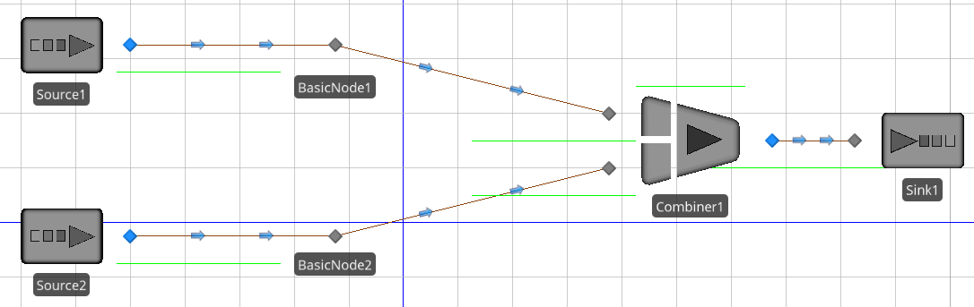
Figure 10.13: Homework problem 2, synchronized system.
Enhance problem 2 so that every entity has an order number and each source creates entities with sequential order numbers starting at 1. We now want to combine only like order numbers, so we must now synchronize entities with identical order numbers at the basic nodes and only release pairs together.
Consider a manufacturing system illustrated in Figure 10.14 where parts arrive to Receiving approximately 8 minutes apart, are moved by an overhead crane to Grinding, which requires 3-7 minutes. After leaving Grinding, 80% of the time it is moved by crane to shipping, the other 20% of the time it moves by crane to Rework. Parts leaving Rework always return by crane to Grinding. The single overhead crane normally parks near Receiving when idle. It has a load and unload time of 1.0 minute, and a lateral movement speed of 1.0 meters per second. Run the model for five 24-hour days and determine the expected utilization of the crane and the machines.
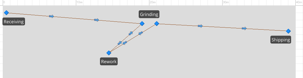
Figure 10.14: Homework problem 4, crane system.
Assume that we want to increase production in the system described in problem 4. If we add a second identical crane to be parked at the opposite end when idle, and add a second unit of Grinding capacity, what is a reasonable receiving rate that could be supported? What changes would you suggest to increase that throughput?
Model a small clinic where the entrance/exit is on the first floor but the doctors office (3 doctors) is on the second floor. Patients arrive at a rate of approximately 30 per hour throughout the 8 hour day. A bank of two elevators each with a capacity of 4 people carries passengers between floors. The patients see one of the doctors for between 3 to 7 minutes, then travel back to the first floor exit. Use the Elevator objects from the Extras library to help model this.