Simulation Modeling with Simio - 6th Edition
Chapter
5
Data-Based Modeling: Manufacturing Cell
Most simulation models employ substantial amounts of data in their development and execution. In SIMIO, employing a data table, as seen in the previous chapter, provides a convenient means to store and recall the data. In this chapter, we will use tables more extensively by reconstructing a manufacturing cell consisting of several workstations.
A small manufacturing cell comprises three workstations through which four different types of parts are processed. The workstations A, B, and C are arranged in such a way that the parts must follow the one-way circular pattern, as shown in the layout in Figure 5.1. For instance, if a part is finished at Station C, it would have to travel the distance to Station A and then the distance to Station B before it could travel to where it exits the system. We want to simulate a five-day week with eight hours of operation a day for a total of 40 hours.
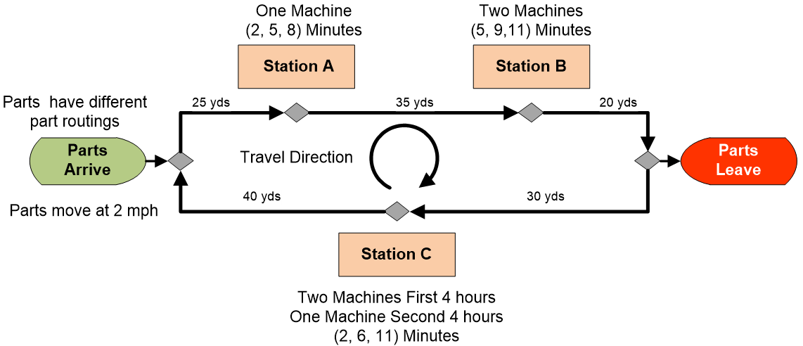
Figure 5.1: Workstation Layout
All parts arrive at the “Parts Arrive” location and leave at the “Parts Leave” location. Travel between workstations is a constant two miles per hour. Note that SIMIO’s default speed for entities is meters per second. The distances (yards) between workstations are shown in Table 5.1 and Figure 5.1.
| WorkStation Path | Distances (yds.) |
|---|---|
| Parts Arrive to Station A | 25 |
| Station A to Station B | 35 |
| Station B to Parts Leave | 20 |
| Parts Leave to Station C | 30 |
| Station C to Parts Arrive | 40 |
Each part type arrives as follows.37
- Part 1’s arrive randomly with an average of 15 minutes between arrivals.
- Part 2’s have an interarrival time that averages 17 minutes with a standard deviation of 3 minutes.
- Part 3’s can arrive with an interarrival time of anywhere from 14 to 18 minutes apart.
- Part 4’s arrive in batches of five exactly 1 hour and 10 minutes apart.
5.0.0.1 What distributions will you choose to model these four arrival processes?
_______________________________________________
Each part (entity) type is sequenced (routed) across the stations differently. In fact, not all part types are routed through all machines, as seen in the sequence order given in Table 5.2.
| Step | 1 | 2 | 3 |
|---|---|---|---|
| Part 1 | Station A | Station C | |
| Part 2 | Station A | Station B | Station C |
| Part 3 | Station A | Station B | |
| Part 4 | Station B | Station C |
Server Properties:
- Station A has one machine with a processing time of two to eight minutes and a likely (modal) time of five minutes.
- Station B has two machines, each with a processing time of five to eleven minutes and a likely time of nine minutes.
- Station C has two machines operating during the first four hours of each day and one operating during the last four hours of the day. Each has a processing time ranging between two and eleven minutes and a mode of six minutes.
5.0.0.2 What distributions will you choose to model the three-station processing times?
_______________________________________________
5.1 Constructing the Model
We will build the SIMIO model using four Sources, three Servers, and several types of links.
5.1.1 Insert four Sources named SrcParts1, SrcParts2, SrcParts3, and SrcPart4 to create the four different part types (i.e., drag four ModelEntities onto the model canvas named EntPart1, EntPart2, EntPart3, and EntPart4).38 Four Sources are necessary because each part has its own arrival process. Make sure to change the Entity Type property of the four Sources to produce the appropriate entity type.
5.1.2 Insert three Servers (i.e., one for each workstation named SrvStationA, SrvStationB, and SrvStationC) and one Sink named SnkPartsLeave. Be sure to name all the objects, including the entities, so it will be easy to recognize them later, as seen in Figure 5.2.
5.1.3 The best method to simulate the circular travel pattern would probably be to use a BasicNode at each station's entry and exit point.39 This allows the entities to follow the sequence pattern without going through an unneeded process. A BasicNode is a simple node to connect two different links, while a TransferNode can connect different links as well but provides the ability to select a destination, path, and/or require a Transporter.
5.1.4 Now connect all the objects using Connectors and Paths. Note that we will use connectors because there is no time lapse or distance between the circular track and the server objects. The distances between stations will be calculated using the five paths connecting each entry and exit node. Be sure that you draw the connectors and paths in the right direction – zoom in on your model to see the “arrows” as shown in Figure 5.2 (i.e., links are entering the input nodes of the Servers while leaving the output nodes).
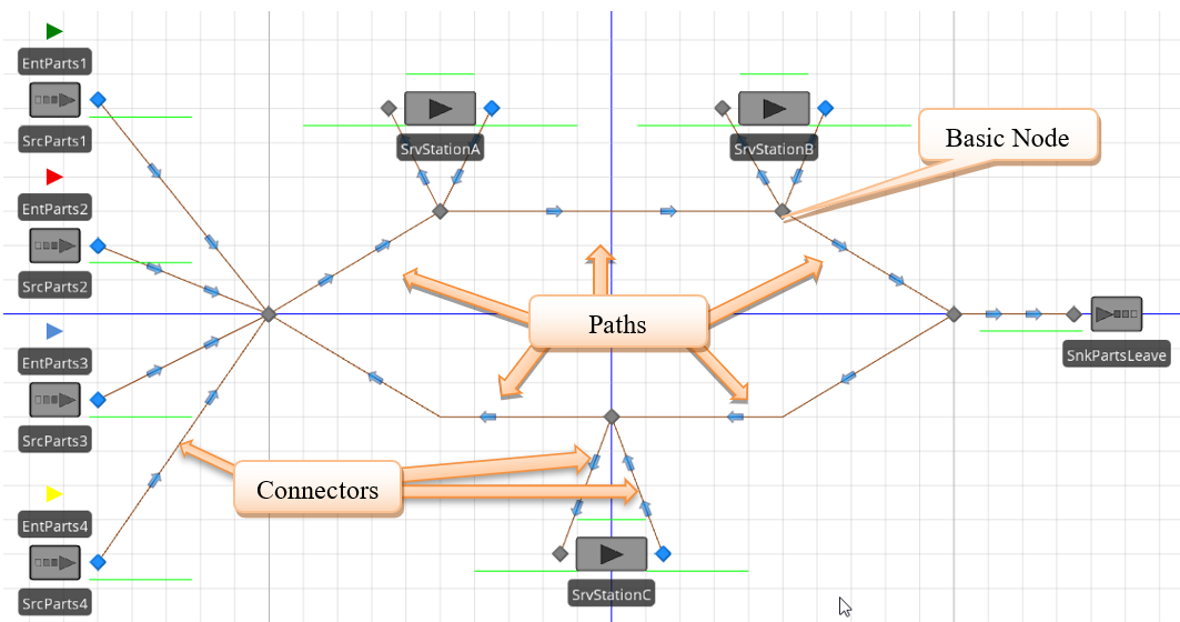
Figure 5.2: Initial Model
5.1.5 Change the properties of each entity so that they now travel at the desired speed of two miles per hour.40 Also, change the color of the entities so you can distinguish between the four-part types by choosing the color on the “Drawing” tab and then selecting the specific entity.
5.1.6 Change the properties of the four source objects so that they correspond to the correct parts and have the desired interarrival times and entities per arrival. We chose Exponential, Normal, and Uniform as the distributions of interarrival times for part types one, two, and three, respectively, with the parameters given. For part type four, we chose a constant interarrival time of 70 minutes and set the Entities Per Arrival property to 5, as seen in Figure 5.3.
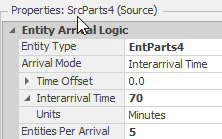
Figure 5.3: Specifying Parameters for the SrcPart4
5.1.7 Set the distances for each of the five paths to correspond to the distances between the stations. You will have to set the Drawn To Scale property for each to “False” to do this and then specify the logical length and units of type”Yards.”
5.1.8 Set the processing times for all the stations using the Pert (BetaPert) distribution. In general, we prefer the Pert distribution to the Triangular distribution. It is specified like the Triangular (minimum, most likely, maximum) but has “thinner” tails, which, we believe, better represents the expected behavior of the processing time distribution. See Appendix A for more information.
5.2 Setting Capacities
We will need to set the capacities for the three workstations, A, B, and C.
5.2.1 Set the capacities for A and B to one and two, respectively. For Station C, we will need to add a work schedule to accommodate the changes in capacity.
5.2.2 Go to the “Data” tab, select “Schedules,” and modify the default schedule (StandardWeek) and the default day pattern (StandardDay). Rename the work schedule to ScheduleForC41 and leave the Start Date property alone to remain the default date on which the simulation will start in the Run setup.
We aim to simulate a five-day week with eight hours of operation a day for a total of 40 hours. Because we do not want to include the idle time (i.e., 12 am to 8 am, 12 pm to 1 pm, and 5 pm to 12 am) in the statistics, we will simulate 40 straight hours, which is equivalent. SIMIO will repeat the work cycle over how many days are in the work pattern. Because our simulation will start at 12 am and run for 40 hours, we want to set the Days in Work Schedule property to 1 and let the cycle repeat after the first 24 hours.
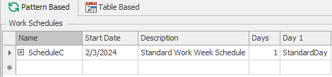
Figure 5.4: Setting up the WorkSchedule
Now select the “Day Patterns” tab to modify the StandardDay day pattern to match the one in Figure 5.5. Change the Start Time property of the first row to 12:00 AM, which will cause the Duration to change to match the End Time. Change it back to “4 hours” and click the Enter. After changing the capacity value to two, repeat this process for the second row using one as the capacity value. Next, add four new work periods by specifying the Start Time, the Duration, and the capacity value.
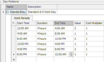
Figure 5.5: Modifying the Day Pattern to Represent Three Eight-Hour Days
5.2.3 Go back to the “Facility” tab and set the Capacity Type property of Station C to “WorkSchedule” using your work schedule, namely ScheduleForC.
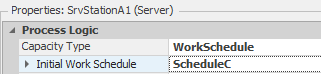
Figure 5.6: Specifying the WorkSchedule for the StationC
5.3 Incorporating Sequences
The way the current model is set up, entities will branch at nodes based on link weights and the direction of the link. However, we want the entities to follow a desired sequence of stations as seen in Table 5.2. We want to be sure that entities will continue along the circular pattern until they reach the node that takes them to their particular station. To accomplish this, we will use “Sequence Tables” (from the “Data” tab).
5.3.1 Click the “Add Sequence Table” button under the drop-down from “Add Table” in the “Data” tab, as seen in Figure 5.7, and rename the new table SequencePart1 to correspond to the first entity type.
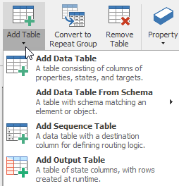
Figure 5.7: Adding a Sequence Table
5.3.2 Now add the sequence of nodes that you want Part 1 to follow (i.e., Station A, Station C, and Exit). You only need to include the visited nodes at each station and the exit. Once the entity’s sequence has been set, it will always travel the shortest route to get to the first node on the list. The correct sequence for Part1 is given in Figure 5.8.42
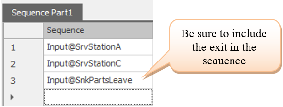
Figure 5.8: Sequence for Part1
5.3.3 Next, add three more sequence tables to correspond to the remaining three entities (i.e., SequencePart2, SequencePart3, and SequencePart4). Set the sequences for each of the other three parts in their corresponding sequence tables as well. Make sure the last node is associated with the Sink. Note that the stations' names may appear differently in your sequence if you name them differently.
5.3.4 Return to the “Facility” tab and click on the EntPart1 entity. Set the Initial Sequence property to the “SequencePart1” under the “Routing Logic” section, which you just created for “Part 1,” as seen in Figure 5.8. Please do the same for each of the other entity types and their associated sequences.
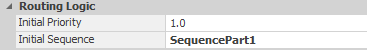
Figure 5.9: Specifying an Entity to follow a Particular Sequence
5.3.5 Do the same for each entity type and their associated sequence. A better method is to use the “Properties Spreadsheet,” as seen inFigure 5.10. Right-click one of the ModelEntities and select the “Object Property Spreadsheet” button. Next, select the “Routing Logic” tab and specify each entity's sequence table.
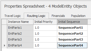
Figure 5.10: Using the Properties Spreadsheet to Set Properties of All Four Entities
5.3.6 For each of the seven TransferNodes (i.e., the output nodes at each source and server), change the Entity Destination Type property from “Continue” to “By Sequence” for each one.43 The first time an entity passes through a transfer node where its destination is “By Sequence,” the node sets the destination of the entity to the first row index of the Sequence Table. After that, every time an entity passes through a transfer node with the “By Sequence” destination type, the row index of the table is increased by one, and the destination of the entity is set to the next node in the table.44
| Type | Definition |
|---|---|

|
Simple node to support the connection between links. Often used for Input nodes of objects (e.g., Sink , Server , etc.). |

|
Supports connection between links but has the ability to select entity destination as well as request a transporter. Output nodes of objects ( Source , Server , etc.) are TransferNodes . |
5.4 Embellishment: New Arrival Pattern and Processing Times
We now learn that the parts arrive in one stream of arrivals (i.e., with a mean arrival rate of 6 per hour, Poisson distributed45) instead of four. There are still four-part types, but the type is random based on the percentages specified in Table 5.4. The number of each that arrives doesn’t change (i.e., meaning Part 4 arrives five at a time).
| Part Type | Percentages | Number to Arrive |
|---|---|---|
| Part 1 | 25% | 1 |
| Part 2 | 35% | 1 |
| Part 3 | 25% | 1 |
| Part 4 | 15% | 5 |
5.4.0.1 When do you think using a single source to model entity arrivals is preferred over multiple sources?
_______________________________________________
Previously, the processing times at the various stations were the same regardless of the part type. Now, we discover that the processing times depend on the particular part type, as shown in Table 5.5. In this table, the sequences are the same as before, but the processing times have been added here.
| Step | 1 | 2 | 3 |
|---|---|---|---|
| Part 1 | Station A (Pert (2,5,8)) | Station C (Pert(2,6,11)) | |
| Part 2 | Station A (Pert (1,3,4)) | Station B (Uniform (5 to 11) | Station C (Uniform (2 to 11)) |
| Part 3 | Station A (Triangular (2,5,8)) | Station B (Triangular (5,9,11)) | |
| Part 4 | Station B (Pert(5,9,11)) | Station C (Triangular (2,6,11)) |
5.4.0.2 Do you think that it is realistic that the processing time for Part 1 on Station A might be different for Part 2 on that same Station A?
_______________________________________________
5.4.1 Now delete all but one of the Sources referring to Figure 5.11 as an example and rename the one Source as SrcParts. We will return to specifying this source after we specify the processing times.
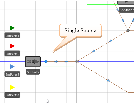
Figure 5.11: Manufacturing Cell Model
5.4.2 The processing times will be added to the original sequencing tables to model the processing times, which are dependent on the part type. When the entity is assigned a destination (i.e., a row in the sequence table is selected), the processing time column can be accessed for that row. (Note: you could use a more complicated expression for the processing time by checking to see if this is a Part A, then make the processing time X, etc., but it is not very easy if there is a large number of parts).
5.4.3 Go to the “Data” tab and click on the SequencePart1 table, which is associated with Part 1 types. Since the processing times can be any distribution (i.e., any valid expression), add a new Expression type column from the Standard Property drop-down named ProcessingTimes. Ensure the column has the appropriate units by making the Unit Type “Time” and the Default Units “Minutes.”
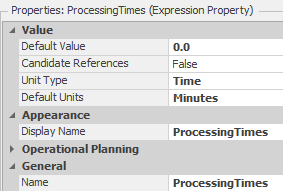
Figure 5.12: Adding an Expression Column to the Sequence Tables
5.4.4 Set the Processing times for SrvStationA (i.e., the first row) to a Random.Pert(2,5,8), SrvStationC (i.e., the second row) to a Random.Pert(2,6,11) and finally, the SnkPartsLeave or third row will remain zero, as seen in Figure 5.13.
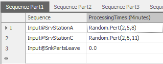
Figure 5.13: New Sequence Table for Part Type 1
5.4.5 Repeat the last two steps for the remaining three-part sequence tables using the appropriate processing times from Table 5.5.
5.4.6 In order to have a single source produce multiple types of entities, a new data table has to be created to specify the part type entities and the part mix percentages. Add a new data table called TableParts with four columns with the specified types, as seen in Table 5.6.
| Column | Column Name | Column Type |
|---|---|---|
| 1 | PartType | Object Reference Property → Entity |
| 2 | ProcessingTimes | Property → Expression |
| 3 | PartMix | Property → Integer (or Real) |
| 4 | NumberToArrive | Property → Integer (or Real) |
5.4.7 Next, specify each entity as a new row with the appropriate processing times, part mix percentages, and sequence table as shown in Figure 5.14.
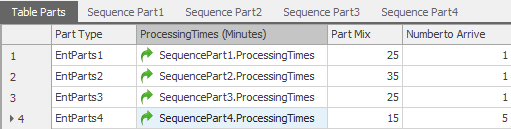
Figure 5.14: Order Type Symbol and Percentages
Specifying SequencePart1.ProcessingTimes states that the processing time will come from the column associated with ProcessingTimes in the table SequencePart1 for the current row.
5.4.8 In order to use the dependent processing times, change each of the processing time expressions in the three stations to TableParts.ProcessingTime. This logic specifies that the processingtime will come from the ProcessingTimes column of the data table TableParts. As the parts move through their individual sequence table (i.e., row to row), it will retrieve the processing time for the current row. The property is now a reference property type  which can only be changed back to a regular property by right-clicking on the label (i.e., Processing Time) and resetting it.
5.4.9 The Entity Type must be changed from a specific entity type to generate multiple part types from the same source. In theSource, specify the Entity Type to come from the TableParts.PartType. This will allow the Entity Type to come from one of the four entities defined in the table.
5.4.10 Set the interarrival time of entities to be an Exponential with a mean of ten minutes (i.e., same as a Poisson arrival rate of six per hour). Set the Entities Per Arrival to TableParts.NumberToArrive.
5.4.11 The part mix percentages will be utilized to determine which specific part type is created. The Source has a property category called “Table Reference Assignment,” which can assign a table and a row of that table to the entity.46 There are two possible assignments: Before Creating Entities and On Created Entity. We want to do the assignment before the entity is actually created so that the Source can create the correct entity type and number to arrive. Therefore, specify the table shown in Figure 5.15.
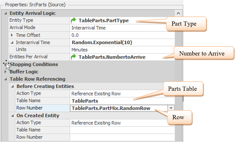
Figure 5.15: Making the Table Reference Assignment
You specify which table (e.g., TableParts) and which row in the table to associate with the object. In this case, the row is determined randomly by using the PartMix column and specifying that a random row should be generated (TableParts.PartMix.RandomRow.47
5.4.12 Save and run the simulation model for 40 hours at a slow speed to ensure each part follows its sequence appropriately and answer the following questions.
5.4.12.1 How long is each part type in the system (enter to leave)?
_______________________________________________
5.5 Using Relational Tables
The original model utilized just four-part types; however, we may need to add additional parts. This would require adding a new entity and rows into the TableParts and creating a new sequence table for each new part. Each addition now requires design time to continue updating the model and adding sequence tables. Instead, can we drive these specifications from a spreadsheet containing the number of parts and their sequences? Or is there an easier way to implement the creation and sequencing of parts?
One inventive modeling construct in SIMIO is using relational data tables. SIMIO has implemented limited database capabilities that can facilitate the modeling of relationships. Figure 5.16 shows a “relational diagram”48 where the TableParts data table is related to the SequencePart Table via the ID column. ID is a primary key (PK) in the TableParts, which uniquely identifies each row in the table (i.e., there cannot be any duplicates). The child table (i.e., SequencePart) inherits the primary key from the parent table (i.e., TableParts), which is denoted as a foreign key (FK). A particular part can have many rows (records) in the child table.
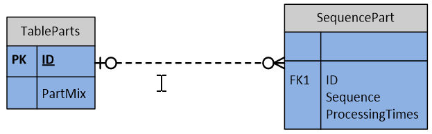
Figure 5.16: Setting up a Relation between Table Parts
5.5.1 First, we will no longer need just four-part types since we want to make this a more generic model. Delete all but one of the part-typeentities and rename the remaining entity EntParts. Add five additional symbols from the Additional Symbols section, making sure to color each new entity as seen in the rotated Figure 5.17.49
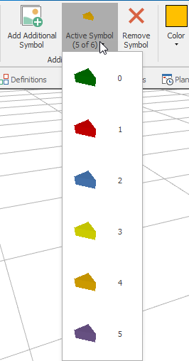
Figure 5.17: Adding Additional Symbols for the Part Entity
5.5.2 For the SrcParts, set the Entity Type property to EntParts.50
5.5.3 From the Data tab, delete all the columns of the TableParts except for the Part Mix and Number to Arrive columns. Insert a new Integer Standard Property named ID. From the Edit Column section, you can move the new column to the left and set the column as a PK using the Set Column As Key button in the same section, as seen in Figure 5.18. Set the ID for each part type to a unique number (i.e., 1, 2, 3, and 4).
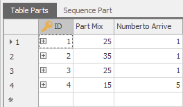
Figure 5.18: Parent Table TableParts with the ID as Primary Key
5.5.4 Select the SequencePart1 sequence table and rename it SequencePart. From the Columns section, select the Foreign Key Property button. Set the properties for the column to specify TableParts.ID is the primary table key to relate the column, too, as seen in Figure 5.19. Change the name of the column to ID.
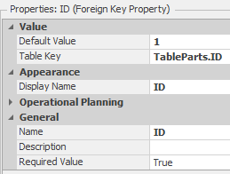
Figure 5.19: Specifying the Foreign Key Property
5.5.6 Select the SequencePart2 tab and then highlight all the rows by selecting the first row using the row selector and dragging it down. Then, copy all the rows and transverse them back to the SequencePart table. Select the last row and then paste in all the values. Change the IDs of this new part to two.
5.5.7 Repeat for the last two-part sequence tabs, setting their IDs to three and four, respectively, as seen in Figure 5.20.
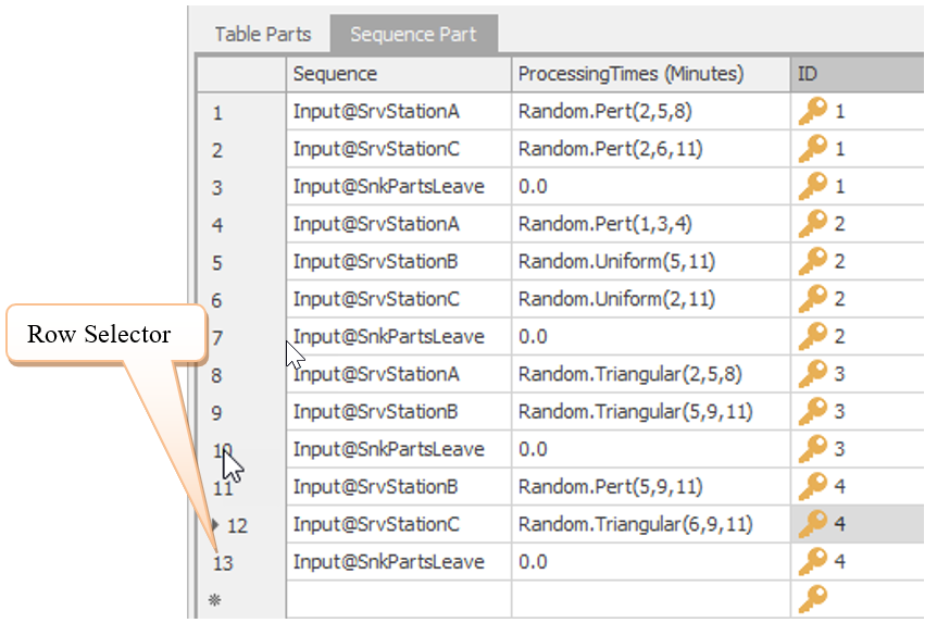
Figure 5.20: The New Sequence Parts Table
5.5.8 Once the table is set up, select the TableParts table again and observe that each row now has an expander ( ) associated with it. Figure 5.21 shows the related records for “Part type 0.” If an entity is assigned a row from the TableParts table, the related records in the SequencePart table will automatically be assigned.
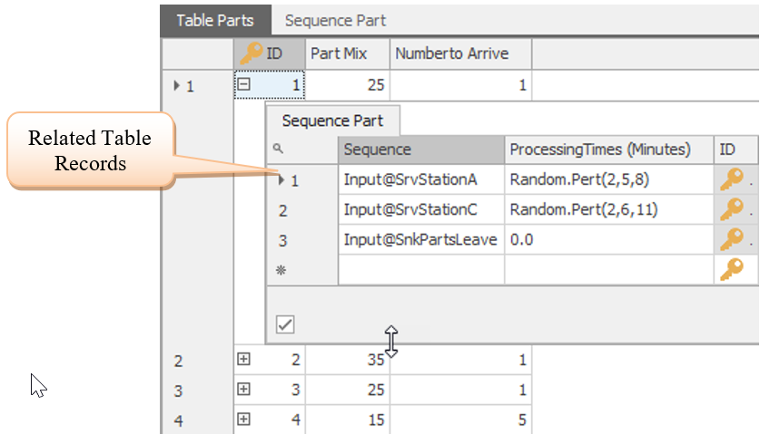
Figure 5.21: Seeing the Related Table Information
5.5.9 We must modify the entity properties to utilize the new sequence table and ID to change the picture symbol. Under the Animation section, change the Current Symbol Index to “TableParts.ID-1” so the color will change appropriately and the Dynamic Label Text to “TableParts.ID-1.”51 Also, ensure the Initial Sequence Property is set to “SequencePart,“ as seen in Figure 5.22. Note that the entity will only receive the related records, not the entire SequencePart table.
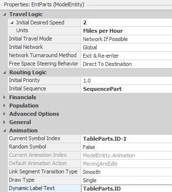
Figure 5.22: Modifying the EntParts Property to Utilize the New Tables
5.6 Creating Statistics
SIMIO automatically produces statistics for various objects within the simulation. For example, statistics are automatically included for the ModelEntity number and time in the system. For any server, there is a scheduled utilization, a number in the InputBuffer station, the waiting time in the station, etc. However, despite their comprehensive nature, that may be insufficient. For example, our latest model has only one entity type, so the ModelEntity statistics are not separated by the part type. What if we wanted to know, on average, how many Part 3’s are in the system during simulation, and what is the average time these parts spend in the system?
The two major statistical categories are Tally statistics and State statistics. The Tally statistic is based on observations like waiting time, time in the system, cycle time, etc. The State statistic, such as number in queue, number in inventory, etc., is a time-weighted statistic such that the time a value persists is used to compute the statistical value. While the State statistic may appear to be the more complicated, it is the easiest to specify in SIMIO. For example, let’s add a State statistic to determine the average number of Part 3’s in the system first and then add a Tally statistic for the average times in the system.
5.6.1 Before creating a State statistic, it is necessary to create a state variable that will hold the values, for example, the number of Part 3’s in the system. SIMIO will monitor the value of the state variable through a State statistic and weight its value according to the time a particular value persists throughout the simulation. Since the number of Part 3’s in the system is a model-based characteristic and not associated with a particular entity, we need to define a model-based state variable. From the Definitions→States section, insert a new Discrete Integer variable with the name GStaPart3NumberInSystem, as seen in Figure 5.23
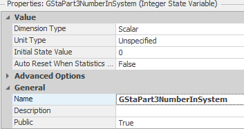
Figure 5.23: Discrete, Integer, Model-based State Variable
5.6.2 The variable needs to be incremented when a Part 3 enters the system and then decremented when a Part 3 leaves the system. Let’s use the State Assignments of the SrcParts for Before Exiting, employing the Repeating Property Editor to increment the new state variable, as shown in Figure 5.24.
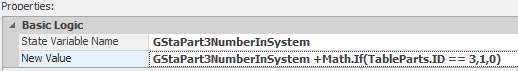
Figure 5.24: Incrementing the State Variable
5.6.3 The Math.If() function simply tests if the r fontc(“TableParts.ID”)` has the value of “3,” which refers to Part 3’s, then adds “1” to the state variable, otherwise, the expression adds “0.”
5.6.4 In a similar fashion, the state variable can be decremented in the State Assignments of the SnkPartsLeave for On Entering, as shown in Figure 5.25.
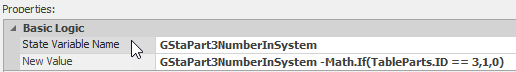
Figure 5.25: Decrementing the State Variable
5.6.5 Now all you need to do is to insert StateStatistic from the Definitions→Elements section named StateStatNumberPart3InSystem that watches the state variable asseen Figure 5.26.
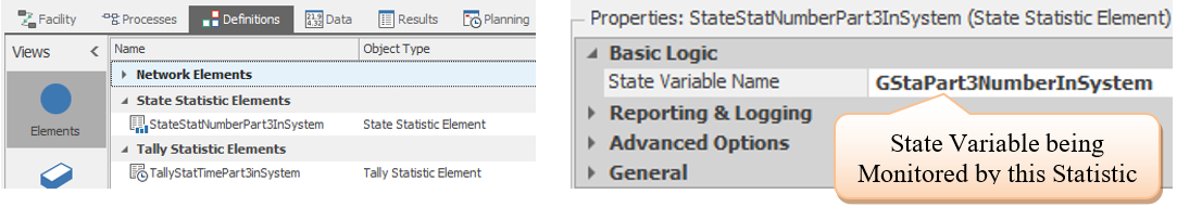
Figure 5.26: Defining the State Statistic Element
5.6.7 Now, we would like to collect time in system for the Part 3’s, which is a Tally statistic. The tally statistic needs to record individual observations. Tally statistics can be collected at any Basic or Transfer node in their Tally Statistics property.52 Unlike the State statistics, the Tally statistic needs to be defined first. Using the Definitions→Elements section, insert a Tally Statistic named TallyStatTimePart3InSystem. See Figure 5.27 for specifying the Unit Type property of “Time.”
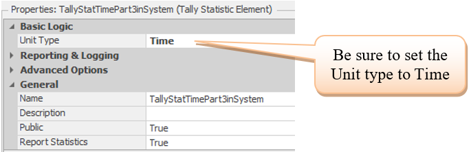
Figure 5.27: Defining the Tally Statistic Element
5.6.8 Select the Input@SnkPartsLeave node (i.e., the one attached to thesink). Under the Tally Statistics Section, using the On Entering tally property, specify which observation (i.e., ModelEntity.TimeInSystem) to record using the Repeating Property Editor. Specify the collection of the tally statistic as shown in Figure 5.28.
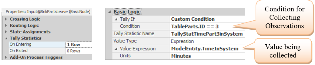
Figure 5.28: Specifying the Collection of Part 3 Time in the System
5.7 Obtaining Statistics for All Part Types
Since statistics like time and number in the system would be useful for each part type, we will extend the statistics collection to all part types rather than just Part 3’s.
5.7.1 First, let’s create the time in system statistics. Navigate to the Definitions→States section and modify the definition of GStaPart3NumberInSystem. Rename the variable to GStaPartNumberInSystem. Set the Dimension Type property of the state variable to a “Vector” with “4” rows, as shown in Figure 5.29. This will create a vector of four state variables, one for each part type.
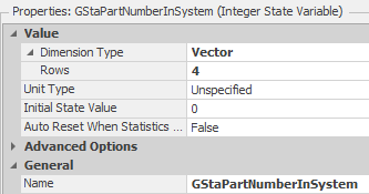
Figure 5.29: Defining the Number in System Vector
5.7.2 Next, change the state assignments at SrcParts and SnkPartsLeave to increment and decrement the number in the system for each part type, respectively, as shown in Figure 5.30. Note that the row (TableParts.ID is used in the vector and [] to access the row in the vector in the expression.53

Figure 5.30: Incrementing and Decrementing the Number in System
5.7.3 You can now define state statistics for all the parts. Under Definitions→States, create three more state statistics named StateStatNumberPart1InSystem, StateStatNumberPart2InSystem, and StateStatNumberPart4InSystem. You need to specify the state variable for each of the statistics using the previously defined vector state variable. This specification is the same for each statistic except for the row. The specification for Part 2 is shown in Figure 5.31. Modify all the four state statistics.
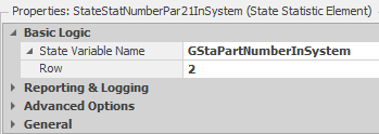
Figure 5.31: Specification for StateStatNumberPart2InSystem
5.7.4 Now define the Tally statistics for the other three-part types (Parts 1, 2, and 4), just as was done for TallyStateTimePart3InSystem (see Figure 5.27 making sure the Unit Type property is equal to “Time.”
5.7.5 Navigate to the Data→Tables section and select the TableParts Data Table. Insert a new Tally Statistic Element Reference property named TallyStatTimeinSystem, allowing us to specify a tally statistic for each part. Therefore, each entity (i.e., part type) will know which statistic to update. There is little need to insert State statistics into the data table since we don’t reference them within the model – only the state variable that the state statistics monitor. Fill in the tables as shown in Figure 5.32.
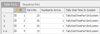
Figure 5.32: Data Table Including Tally Statistics
5.7.6 Once the Table row reference has been assigned, each ModelEntity (i.e., part) will have an associated Tally statistic, eliminating the use of complicated deciding logic when determining which Tally statistic to update. Select the Input@SnkPartLeave Basic node in front of SnkPartLeave, and under the Tally Statistics entry, click on On Exited.54 Use the Tally Statistic Name based on the row that has been assigned to the entity (i.e., TableParts.TallyStatTimeinSystem. The observation Value will be the model entity time in system value, as seen in Figure 5.33, to utilize the entity’s tally statistic.
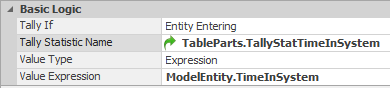
Figure 5.33: Time in System Tally Statistics
5.7.7 Now, re-run the simulation and examine the results.
5.7.7.1 Are the tally statistics on time in the system for each part type the same as the results from Part 5.4:?
_______________________________________________
5.7.7.2 Do the state statistics for the number in the system for each part match the results from Part 5.4:?
_______________________________________________
5.8 Automating the Creation of Elements for Statistics Collection
Adding intelligence to entities made it easy to model different routings and calculate time in the system and number in system statistics for each part type without creating multiple sink and source objects corresponding to the individual parts. However, we would still need to define the associated statistic objects and state variables. Such an approach becomes very cumbersome if we want to add many new part types.
An advantage of using related tables is that they may be linked (bound) directly to a spreadsheet containing many part types and sequences. Nevertheless, we may want statistics for time in the system (i.e., cycle times) and the number in the system for each part type. However, each part type will require a Tally and State statistic. Having to define each statistic could negate the advantages of using related tables as individual tally and state statistic elements need to be created, and the correct statistic must be collected for the particular part. However, SIMIO allows for the automatic creation of state variables and statistic elements.
5.8.1 If you are using the model from the previous section, you should delete all the Tally and State Statistic elements so these can be created automatically.
5.8.2 Since the number of part types might change, the state variable GStaPartNumberInSystem must be modified to match the number of parts in the table each time. In our case, we must set it equal to the maximum possible number of part types in the system (e.g., 10).55 The size of the state variable can be tied to the number of rows and columns of a data table. From the Definitions→States section, change the Rows property from “4” to “10”.
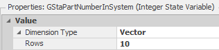
Figure 5.34: Specifying the Size of the State Variable to Match the Table
5.8.3 Navigate to the Data→Tables section and select the TableParts Data Table. Insert an Element Reference Property→Tally Statistic property named TallyStatTimeinSystem. Remove the tally statistics from that column, so it looks like Figure 5.35. Note that the tally statistics references are missing.
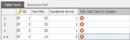
Figure 5.35: Adding a Tally Stat Reference Column
5.8.4 Once one specifies entries (i.e., names), the elements will be created. The element’s initial properties can be manually specified (e.g., Category, Data Item, Unit Type, etc.) from the Definitions→Elements section. However, since the number of part types can be dynamic, we do not want to have to specify these properties each time, which would defeat the benefit of automatic specification of the statistical elements. Therefore, the elements that are created can also have their properties initialized by specifying another column in the table as their values. For our problem, the category and data item classification of the Tally statistics can be specified as we want it to be the same as other time in system statistics (i.e., “FlowTime” and “TimeInSystem”). Therefore, insert two standard Property→String property columns named Category and DataItem, as seen in Figure 5.36.
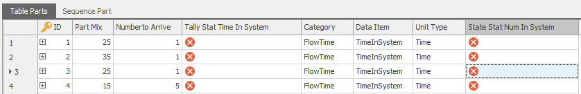
Figure 5.36: Adding Properties to the Statistical Elements
5.8.5 For the Unit Type property of the Tally statistic, insert a standard Enumeration property column named UnitType into TableParts, as was done in Figure 5.36. An enumeration is a property whose value is specified from a list of potential values. In this case, unit types can be “Unspecified,” “Time,” “Length,” etc. For the Enumeration column property, specify the Enum Type as “UnitType” to pull its values from the unit type enumeration list. Then, the Default Value should be “Time,” as seen in Figure 5.37.
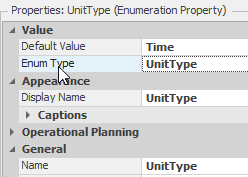
Figure 5.37: Setting up the Enumeration Property Column
5.8.6 Next, insert a State Statistic Element Reference property named StateStatNuminSystem, as seen in Figure 5.36.
5.8.7 Rather than creating each Tally and State statistic to specify as entry values, SIMIO has the ability to automatically create elements (i.e., Tally and State statistics, Materials, etc.) specified from a table column. Therefore, each part row can have a specified Tally statistic (i.e., name) that will automatically be created and used to keep track of its on-time in system statistics. By default, the Element Reference property column will be of a “Reference” type, meaning the element would need to be already created to be specified as an entry in the table.
- Therefore, change the Reference Type property to “Create,” as shown in Table 5.7 and Figure 5.38.
- Set the Auto-set Table Row Reference property to “True” as well.
| Property | Description and Value |
|---|---|
| Reference Type -Reference | It allows you to specify an element that has already been defined under the “Definitions” tab. |
| Reference Type-Create | Entries in this column will now automatically create a new element of the specified type with the entry’s name. Note that these elements will appear in the Definitions→Elements but cannot be deleted from here. Any name changes in either location (i.e., Table or Definitions→Elements will be reflected in both. |
| Initial Property Values | This can be used to initialize the element based on constants or values in other table columns for that row. |
| Auto-set Table Row Reference | If “True,” then the element that is pointed to by each row will automatically be given a table reference set to that row. If you create and initialize the element based on other columns, this must be the case. |
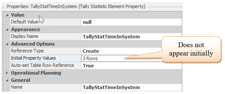
Figure 5.38: Specifying Element Reference to Automatically Create the Element
5.8.8 After specifying the “Create,” the statistical elements will be created, but they will not have their properties referenced. To use the entries specified in these three new columns as the initial properties, select the TallyStatTimeinSystem column and set the Auto-set Table Row Reference to True, which assigns the current row to the newly created element. Next, click the Repeating Property button for the Initial Property Values property. Next, add the following three properties and values as specified in Table 5.8.56 To specify the initial properties, use the repeating property window shown in Figure 5.39.
| Property Name | Value |
|---|---|
| Unit Type | TableParts.UnitType |
| Category | TableParts.Category |
| DataItem | TableParts.DataItem |
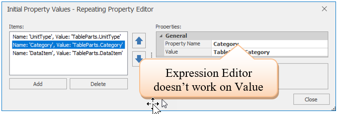
Figure 5.39: Specifying the Initialization Properties of the TallyStat Reference Column
5.8.9 Select the StateStatNumInSystem and specify that this column will be created as well, as seen in Figure 5.40, making sure to set the Auto-set Table Row Reference to True.
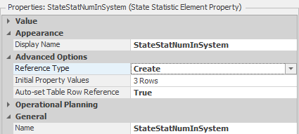
Figure 5.40: Having the State Statistics to be Automatically Created
5.8.10 Next we need to initialize the new state statistics in a similar fashion to the Tally statistic column. However, we will not setup additional columns to specify the parameters. Set the “Category” and “DataItem” properties to string values, and the “StateVariableName” property will use the TableParts.ID to specify which state variable the statistic should monitor as seen in Table 5.9 and Figure 5.41.
| Property Name | Value |
|---|---|
| StateVariableName | GStaPartNumberInSystem[TableParts.Id] |
| Category | Content |
| DataItem | NumberInSystem |
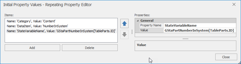
Figure 5.41: Initial Parameters of the State Statistic Column
5.8.11 Add in the specifications for the properties of the four-part types as shown in Figure 5.42.
Figure 5.42: Specifying the Properties of the Statistical Elements
5.8.12 You may now want to reset the Reference Type property back to “Reference.” Then, when you set the Reference Type property back to “Create”, the statistical elements will be automatically created as shown in the Definition→Tally Statistical Elements (Auto-Created) section. Note how each statistic takes its UnitType, Category, and DataItem from the Data Table.
5.8.13 Now, for every new row that is added, a new Tally and State statistic will be created and initialized from the entry values of the Category, DataItem, and UnitType columns. For any rows that existed before the two columns were created, the values will not be initialized.57 We can cut and paste values back and forth from SIMIO tables and Microsoft Excel™ spreadsheets. Select the entire table by highlighting the row selectors and then cut the rows (Ctrl-x). Next, paste them into a Microsoft Excel™ spreadsheet so you don’t have to retype all the information. You can also export the table to a CSV file from the Content tab under the Table Tools section. Modify the names of the tally and state statistics, categories, data items, and unit types, as seen in Figure 5.43.
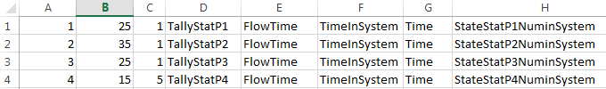
Figure 5.43: Using Excel to Modify the Values
5.8.14 Copy the values in Excel and select the empty row in the SIMIO data table by clicking on the row selector. Then, paste the values into the table, which should now look like the one in Figure 5.35.
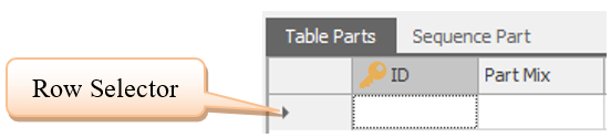
Figure 5.44: Select the Empty Row of a Data Table to Past all Values
5.8.15 Save and run the model for 40 hours.
5.8.16 Now add a fifth part type by creating a sequence and update only the data table (don’t create any elements) by copying the fourth part information (i.e., have the same part mix and number of entities) but changing the ID to 5 and tally and state statistic column values, as well as copying the fourth part sequences for the fifth part.
5.9 Commentary
- The Start Date property of the Work Schedule intuitively would be when the schedule will start. So, if one specified a future date, then nothing would happen until that date. That is not the case. The Start Date property represents the particular day the first day of the pattern will start. If this date is in the future compared to the start of the simulation, it will repeat backwards to the current date based on the pattern. For example, if we have a three-day pattern named Day 1, Day 2, and Day 3, and the work schedule start date is set to 09/17/23, the schedule will follow the Day 1 pattern for this date. If the simulation starts on 09/13/23, then the pattern for 09/13 is Day 3, 09/14 is Day 1, 09/15 is Day 2, 09/16 Day 3, which makes Day 1 on 09/17 and Day 2 on 09/18, etc. To have a work schedule not start until a particular day, exceptions to the workday have to be employed.
- Another way to look at SIMIO properties and states is that property values are established for each object in the Facility window at the beginning of the simulation execution and cannot be changed during “run-time.” In contrast, the value of states is also established at initialization, but it can be changed during “run-time.” Objects that are created during run-time, such as Entity, have their properties established during an instance of run-time, which is during the initialization of that instance. Otherwise, they cannot be changed during the simulation execution.
- Relational tables offer a tremendous advantage over other simulation languages in assigning one table and automatically assigning all records of related tables. We will explore this feature more in later chapters. In later chapters, we will demonstrate how you can bind data tables to Excel spreadsheets, which could facilitate the automatic creation of new parts and sequences.
For the moment, we will let you think about the distributions that these parameters may represent.↩︎
To do this efficiently, drag one Source on to the facility and name it SrcParts. Then copy and paste it three times which will take advantage of the SIMIO naming scheme (i.e., it will create SrcParts1, SrcParts2, and SrcParts3). Now, rename the first source SrcParts4. Repeat this method for the four entities starting with EntPart.↩︎
A TranferNode used to enter/exit from a station can disrupt the SIMIO internal sequencing of sequence steps if one is not careful.↩︎
Select all four entities using the Ctrl button and specify the speed once for all entities.↩︎
Double clicking the Standard Week name will allow you to change the name.↩︎
Note the input nodes of the associated Servers and Sink are specified rather than then actual object. Note the names of the nodes are in the form Input@ObjectName.↩︎
To set them all at once, press the Ctrl key while selecting all seven TransferNodes and then set the Entity Destination to “By Sequence.”↩︎
If the current row index is on the last row and the entity enters a TransferNode that has “By Sequence,” the row index will start over at one. Also, if an entity enters a TransferNode that has “By Sequence,” before reaching the current destination node, the row index will move to the next row in the sequence table.↩︎
Remember that this Poisson arrival rate is equivalent to an Exponential interarrival time with a mean of 10 minutes. SIMIO wants the interarrival time, not the arrival rate – so be prepared to make the conversion.↩︎
In later chapters we will utilize Processes and the Set Row step to assign a table to an entity.↩︎
SIMIO will normalize the numbers so the probability sums to one. Therefore, you may specify whole numbers 25, 25, and 50 rather than percentages 0.25, 0.25, and 0.5.↩︎
More formally it is called an Entity Relationship Diagram, but the word “Entity” is use differently than it is used in SIMIO.↩︎
Note the symbols start with “0” index.↩︎
Right click the property and reset it back from the reference property.↩︎
If we had a lot of parts, we can utilize just the Dynamic Label Text to display the ID as the part moves through the network making this work for any number of parts. This concept will be explored in later chapters.↩︎
In later chapters we will use the Tally process steps to collect statistics anywhere.↩︎
The row index of the first row for Vectors, Matrices, and Data Tables is one while symbol indexes start at zero.↩︎
The On Entering could be used as well.↩︎
“Matrix from Table” is another Dimension Type for state variables which will create a two dimensional matrix based on the number of rows and numeric columns of a table. Dynamically. However, it initializes the variable based on the table values.↩︎
You will need to type in the values directly as this is not an expression editor.↩︎
We can either modify the properties our self or we can delete the rows and recreate them. You can select the AutoCreate dropdown in each column value.↩︎