Simulation Modeling with Simio - 6th Edition
Chapter
16
Modeling of Call Centers
Workschedules, non-homogenous rate tables, and routing have already been extensively used in previous chapters. This chapter will reinforce those concepts while demonstrating how to handle two of the most common behaviors of people in queues: “balking” and “reneging.”
A call center receives support calls from customers who purchase kitchen appliances. The call center is open seven days a week from 8:00 am to 7:00 pm (i.e., 11 hours). It is, however, staffed from 8:00 am to 8:00 pm, which leaves an hour to finish calls that are in process at 7 pm. There are two lines for technician service. Customers are routed to the technicians (see Figure 16.1) depending on whether or not the first line can answer the customer’s questions.
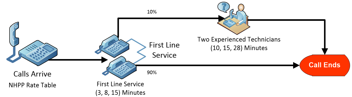
Figure 16.1: Model of a Simple Call Center
Information about the arrival rate of calls during the day is available. Table 16.1 (taken from historical data) displays how the call rates change from hour to hour during the 12-hour day. Note that no calls are taken during the last hour.
| Time Interval | Hourly Rate |
|---|---|
| 8 am – 9 am | 35 |
| 9 am – 10 am | 55 |
| 10 am – 11 am | 70 |
| 11 am -12 pm | 85 |
| 12 pm – 1 pm | 95 |
| 1 pm – 2 pm | 110 |
| 2 pm – 3 pm | 90 |
| 3 pm – 4 pm | 88 |
| 4 pm – 5 pm | 60 |
| 5 pm – 6 pm | 50 |
| 6 pm – 7 pm | 30 |
| 7 pm – 8 pm | 0 |
Calls are serviced in the order they are received at the call center, and ten support technicians answer the calls. Apparently, the time it takes to answer a call generally takes 8 minutes to answer a support question, with a minimum of 3 minutes and a maximum of 15 minutes. The first-line service technicians can completely answer ninety percent of the calls. So, after working with the customer on the original question, ten percent of the calls must be routed to more experienced technicians, of which there are two technicians. The second-line technicians end up taking about 15 minutes on the call, with a minimum of 10 and a maximum of 28 minutes.
Since the call center uses telephonic equipment, the calls are transferred automatically to the service centers. And, to the best of our knowledge, once a call comes in, the customer stays on the line until it is processed (i.e., currently, there are no call abandonments). When we were able to talk with people at the call center, we found that staffing was not constant throughout the 12-hour day, but there were a number of different schedules for the workers, including part-time and full-time. In fact, the work schedule is described in Table 16.2.
| Time Period | Number of First Line Technicians |
|---|---|
| 8 am – 9 am | 5 |
| 9 am – 10 am | 5 |
| 10 am – 11 am | 8 |
| 11 am -12 pm | 10 |
| 12 pm – 1 pm | 10 |
| 1 pm – 2 pm | 16 |
| 2 pm – 3 pm | 16 |
| 3 pm – 4 pm | 12 |
| 4 pm – 5 pm | 8 |
| 5 pm – 6 pm | 8 |
| 6 pm – 7 pm | 8 |
| 7 pm – 8 pm | 2 |
16.1 Building the Simple Model
16.1.1 Create a new model with one Source named SrcCallsArrive, a Sink named SnkCallsExit, and two Servers named SrvFirstLineTech and SrvAdvancedTech, as well as add a ModelEntity named EntCalls as shown in Figure 16.2.
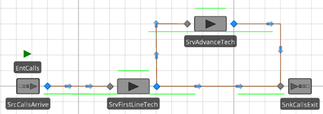
Figure 16.2: SIMIO Model of a Simple Call Center
16.1.2 Connect all of the objects via Connectors since these are electronically switched calls. To handle the case that 10% of the calls have to be routed to the advanced technical support line, specify a selection weight of 10 for the connector linking SrvFirstLineTech to SrvAdvanceTech and a selection weight of 90 for the connector between the SrvFirstLineTech and SnkCallsExit.
16.1.3 From the Data→Rate Tables section, create a new Rate Table named RateCallTable with 12 intervals and a one-hour interval size as shown in Figure 16.3.249
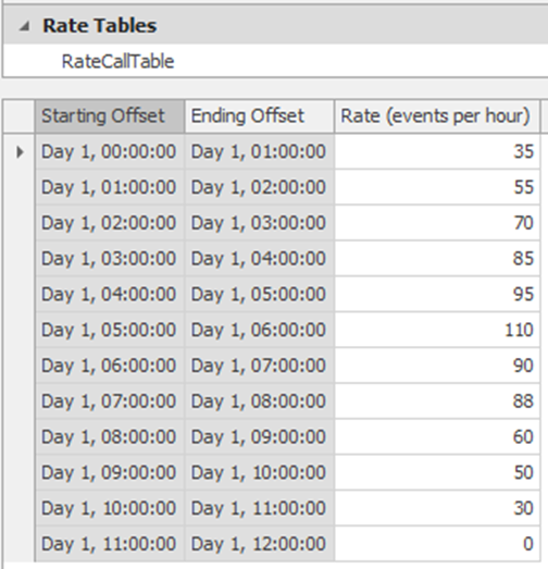
Figure 16.3: Arrival Rate Table for the Call Center
16.1.4 Return to the model and change the Arrival Mode property of the SrcCallsArrive source to “Time Varying Arrival Rate” and specify the RateCallTable as the Rate Table property (Figure 16.4).
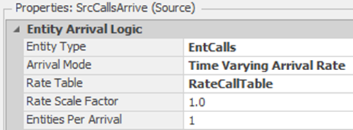
Figure 16.4: Specifying the Arrival Mode of the Call Arrival Source
16.1.5 Select the SrvAdvanceTech server, change the Initial Capacity property to two, and set the Processing Time property to Random.Pert(10,15,28), which will simulate two advanced technicians.
16.1.6 Next, the work schedule of the first-line technicians needs to be created. Recall that SIMIO already defines a default work schedule and day pattern for you. Select the “StandardDay” pattern from the “Day Patterns” tab under the Data→Schedules section and modify it to match the data in Figure 16.5.250 Let us use the WorkSchedule on the left as it specifies every hour separately versus the one on the right, which groups some time periods into one for the same values. We will need each time period in a subsequent section.
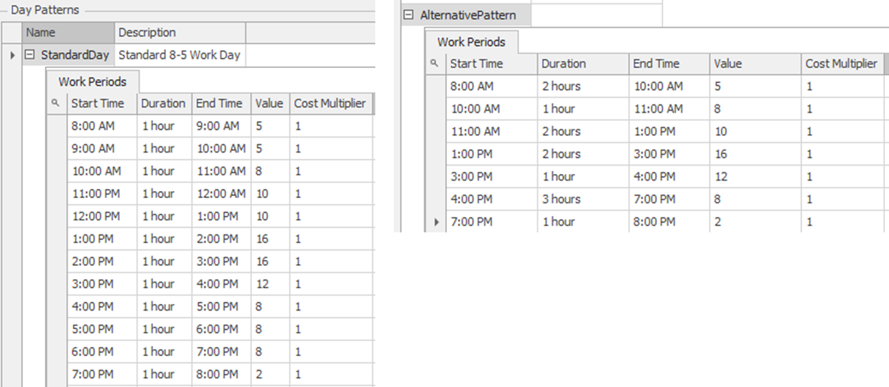
Figure 16.5: Work Schedule for the First Line Technicians
16.1.7 Return to the Model, select the SrvFirstLineTech, and specify the new work schedule and processing time, as seen in Figure 16.6.
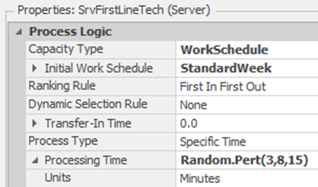
Figure 16.6: Setting the Properties of the First Line Technician Server
16.1.8 Even though we do not allow any more calls to come after 7:00 pm, how many people, on average, will be in the queues at 8:00 pm when there are no more technicians to handle these calls? An Output Statistic can perform this calculation at the end of the simulation run. From the Definitions→Elements, insert a new Output Statistic named OutStatNumberofCallsLeft with the following Expression property: EntCalls.Population.NumberInSystem.
16.1.9 In the Run Setup, change the Starting Time to 8:00 am, and the Ending Type should be 12 Hours. Save and run the model.
16.1.9.1 What is the average customer time in the system, and what is the number of calls still at the end of the simulation?
_______________________________________________
16.1.9.2 What is the average utilization of the first line and the experienced technicians?
_______________________________________________
16.1.10 Next, insert a new Experiment and run 20 replications of the model.
16.1.10.1 What is the average customer time in the system and the number of calls still in the system at the end of the simulation?
_______________________________________________
16.1.10.2 What is the average utilization of the first line and the experienced technicians?
_______________________________________________
16.2 Balking
Now, you observe that people who may encounter waiting for a service sometimes abandon that service. In queuing theory, this is called “balking.” Effectively, a person who observes the queue as “too long” simply will not join. This scenario is illustrated in Figure 16.7. In our case, the wait time is proportional to the number in the queue, so we will model the waiting time by using the number (or contents) in the queue. If 20 or fewer people are waiting, only 10 % will balk, while 25% will balk when 21 to 30 people are waiting. And finally, if more than 30 people are waiting, the chance of balking is 50%.
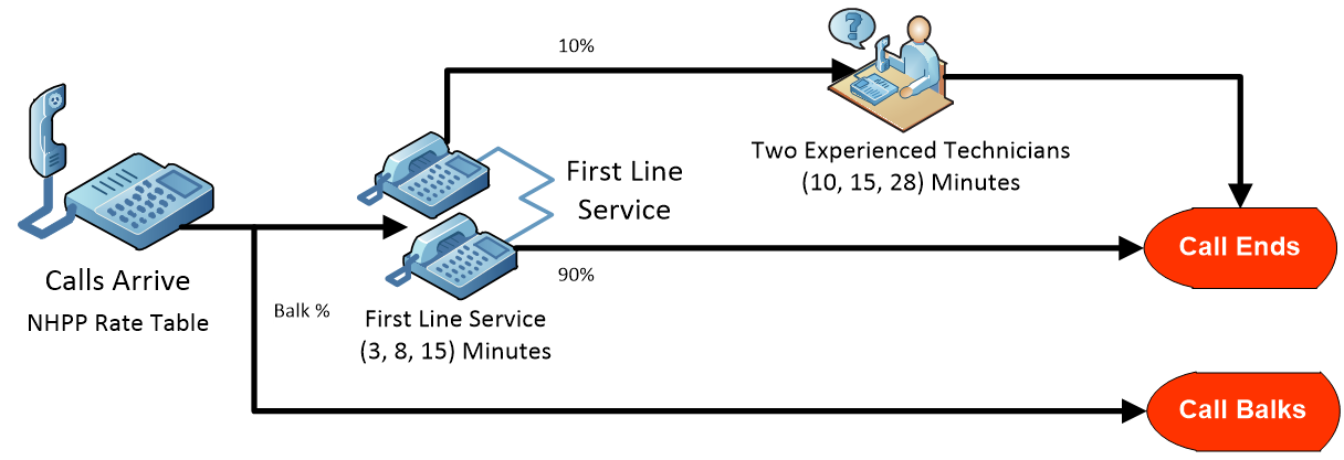
Figure 16.7: Call Center with Balking
16.2.1 Insert a new Sink named SnkBalk below SnkCallsExit and connect the SrcCallsArrive to the new Sink via a Connector.
16.2.2 A Lookup Table offers a great modeling mechanism for predicting the changing balking percentage based on the input queue of the first-line service.251 From the Data tab, create a new Lookup Table named FuncLookupBalkPercent with the appropriate values, as seen in Figure 16.8252.
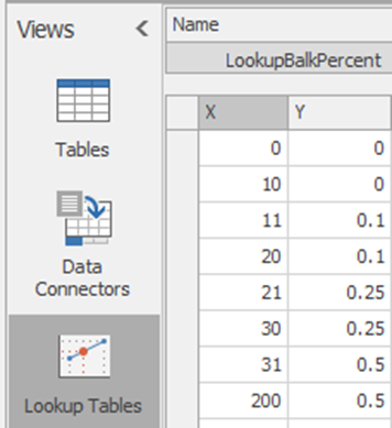
Figure 16.8: Balking Percentage Lookup Table
16.2.3 Since the expression is very long, we will set up a function to make it easier and limit errors from occurring. From the Definitions tab, insert a new function named FuncBalkPercent from the Edit section. Set the following expression to return a value from the Lookup Table based on the number waiting at the SrvFirstLineTech input buffer as shown in Figure 16.9.
LookupBalkPercent[SrvFirstLineTech.InputBuffer.Contents.NumberWaiting]

Figure 16.9: Utilizing a Function
16.2.4 For the connector linking the Source to the Server (SrvFirstLineTech), set the Selection Weight property to 1-FuncBalkPercent and the Selection Weight property of the link connecting the source to the balking sink to FuncBalkPercent.
16.2.5 Save and rerun the experiment.
16.2.5.1 What is the average customer time in the system and the number of calls still in the system?
_______________________________________________
16.2.5.2 What is the average utilization of the first line and the experienced technicians?
_______________________________________________
16.2.5.3 What is the average holding time in minutes for both of the two server’s input buffers?
_______________________________________________
16.3 Modeling Reneging of Customer Calls
Now, we allow customers to renege (i.e., leave) from the queue for standard calls when they have waited for a period of time. In other words, we will allow the abandonment of calls to occur. More specifically, every customer who enters the call queue will wait for at least ten minutes. However, after waiting in the queue for ten minutes, the customer examines its place in the queue (the telephonic system informs them of this). The customer reneges and leaves the system if they are not within the first five places from the front of the queue. If they are within the first five places of the front, then the customer will extend their stay in the queue for another four minutes in hopes of getting served. If they are still in line after the extended stay, they will also renege.
16.3.1 Save the current model and then insert a new Sink named SnkRenege below the SnkBalk, but do not connect it to anything. This sink will be used to collect statistics on those customers who renege.
16.3.2 The modeling methodology to be used is when a call comes into the first-line technician’s service queue. A ten-minute delay occurs, and then we check to see if the call is still in the queue. If it is in the queue and the position is greater than five, they renege; otherwise, you wait another four minutes to see if you have been served. Select the SrvFirstLineTech Server and insert the Entered Add-on Process Trigger.
16.3.3 The actual call ModelEntity would wait ten minutes and then perform the check before entering the server to be placed into the queue or processed. Recall the discussion of how a token associated with the actual ModelEntity invokes the process and executes the steps. In this case, we need one Token to continue through the process (i.e., enter the queue and be processed) while a second Token goes through the delay and for potential removal of the customer from the queue. Figure 16.10 illustrates how an Execute step can be used to spawn a new Token associated (i.e., blue one) with the entity to execute another process. When the first Token associated with the “Call 21” entity runs the Execute step, a new 2nd Token is created that will execute the steps in the new RenegeProcess. The first token can continue, allowing the call to enter the queue and possibly be served.
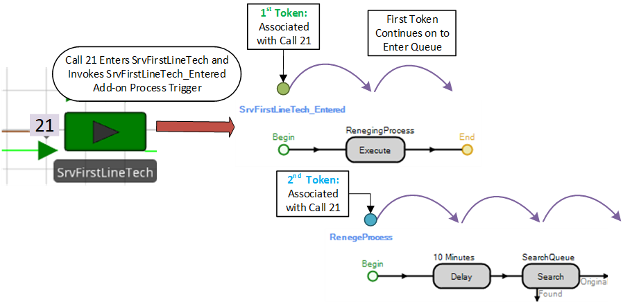
Figure 16.10: Illustrate how Two Tokens are Associated with the Same Call ModelEntity
16.3.4 From the Processes tab, create a new process named RenegeProcess. Under the Advanced Options, set the On Associated Object Destroyed to EndProcess. Refer to Figure 16.11. If the ModelEntity executing the process is destroyed, we want the RenegeProcess to end.253 This will be important if it executes in parallel while the actual entity moves through the network.
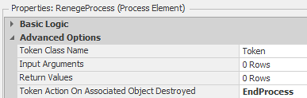
Figure 16.11: Ending the Process if the Entity has been Destroyed
16.3.5 Insert an Execute step into the SrvFirstLineTech_Entered process, as shown in Figure 16.12 which executes the RenegeProcess process. Change the Token Wait Action property to “NoWait” which allows the Token executing this step to continue on. By default it is set to wait until the RenegeProcess finishes, which would not allow the customer to continue to obtain service until the renege process ends (specify the Execute step as shown in Figure 16.12).
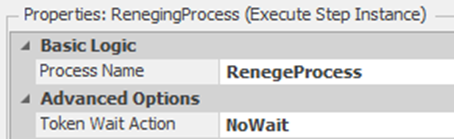
Figure 16.12: Executing the Renege Process but Allowing First Token to Continue
16.3.6 From the Definitions tab, add an Integer Discrete State variable named GStaPosition which will be used to store the position of the caller in the queue.
16.3.7 Return to the “Processes” tab and inset a Delay step into the RenegeProcess,” as seen in Figure 16.13, which delays the Token for ten minutes.254
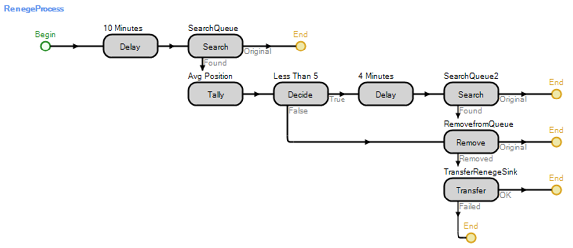
Figure 16.13: Process to Handle Reneging
16.3.8 After the ten-minute delay, we need to check to see if the associated call is still in the queue. If it is in the queue, determine its position. Insert a Search step after the Delay step, which will be used to search the queue and determine its position.255 Change the Collection Type property to “QueueState” and the Queue State Name to SrvFirstLineTech.AllocationQueue. Specify the GStaPosition state variable as the Save Index Found property so it will be assigned the index of the item found. Since we want to search for the associated call in the queue, specify the Match Condition property as ModelEntity.ID == Candidate.ModelEntity.ID, which will search the queue and match the ID of the item in the queue with the associated entity ID, as seen in Figure 16.14.

Figure 16.14: Specifying the Search Step Parameters to Search for the Call in the Service Queue
16.3.9 If the Token associated with the EntCalls ModelEntity finds itself in the queue, then the GStaPosition state variable needs to be checked to see if it is less than or equal to five. Therefore, insert a Decide step that performs a conditional test as shown in Figure 16.15.

Figure 16.15: Checking the Index of the Entity in the Queue
16.3.10 If the entity’s position in the queue is greater than five (i.e., the False branch), we will remove it from the queue and transfer it to the Sink SnkRenege. Insert a Remove step on the “False” branch that will remove the current call associated with the “Found” Token from the SrvFirstLineTech.AllocationQueue.256 You will need to type in the value for the Queue State Name property directly if it does not appear in the list.
16.3.11 A Token associated with the removed item will exit out the “Removed” path. Therefore, insert a Transfer step on the “Removed” path to move the entity from the current station to the SnkRenege. The Transfer step details are shown in Figure 16.16.
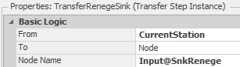
Figure 16.16: Transferring the Reneging Call to the Appropriate Queue
16.3.12 If the position in the queue is less than or equal to five, then delay the Token for an additional four minutes and search again. Insert a Delay step on the “True” path that delays for four minutes.
16.3.13 Copy the first Search step and place it after the four-minute delay to check and see if the entity is still in the queue.
16.3.14 If the call is found in the queue (i.e., it is still waiting to be serviced), it will automatically renege. Grab the  (End) associated with the “Found” path and drag it on top of the Remove step to utilize the same Remove and Transfer steps as seen in Figure 16.13.
16.3.15 For people who have been waiting for over ten minutes to talk with a technician, we would like to know their position after ten minutes on average. From the Definitions→Elements section, insert a new Tally Statistic named TallyStatPosition. In the RenegeProcess, insert a Tally step right before the Decide step. The Tally step details are shown in 16.17.
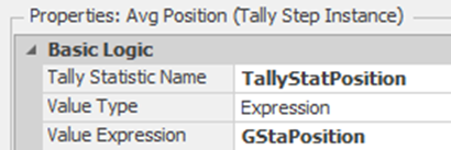
Figure 16.17: Tracking Average Line Position
16.3.16 Save and rerun the Experiment.
16.3.16.1 On average, how many calls renege during the 12-hour simulation run?
_______________________________________________
16.3.16.2 What is the average position for people who have waited at least ten minutes?
_______________________________________________
16.4 Optimizing the Number of First-Line Technicians
We would like to determine if we have enough first-line technicians at the right times to minimize our customers’ costs and wait times. Optimization with OptQuest™ was introduced earlier and will be used again. Sometimes, the WorkSchedules may not be flexible enough, and you may need to resort to another technique. Nevertheless, at the end of the section, we return to specifying properties for the WorkSchedule.
16.4.2 From the Definitions→Properties section, insert 12 Standard Expression Properties with the names and values as seen Table 16.3.257 These properties will be optimized to determine the best number to have during each time period, where TimePeriod1 would correspond to 8-9 AM.
| Expression Property Name | Default Value | Category |
|---|---|---|
| TimePeriod1 | 5 | Call Center |
| TimePeriod2 | 5 | Call Center |
| TimePeriod3 | 8 | Call Center |
| TimePeriod4 | 10 | Call Center |
| TimePeriod5 | 10 | Call Center |
| TimePeriod6 | 16 | Call Center |
| TimePeriod7 | 16 | Call Center |
| TimePeriod8 | 12 | Call Center |
| TimePeriod9 | 8 | Call Center |
| TimePeriod10 | 8 | Call Center |
| TimePeriod11 | 8 | Call Center |
| TimePeriod12 | 2 | Call Center |
16.4.3 Next, insert a new Data Table named TableSchedule under the Data→Tables section, which will become our own manual schedule table, as seen in Figure 16.18.
16.4.5 Insert 12 rows with the value of the expression for each row to be the corresponding property created above, as seen in Figure 16.18.258
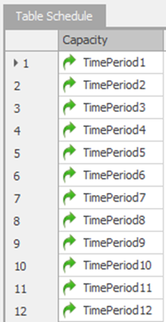
Figure 16.18: Creating our own Work Schedule Table
16.4.6 Since we are creating our own schedule, a Timer will be needed to signal the time to change the capacity of the SrvFirstLineTech server at given intervals. From the Definitions→Elements section, insert a Timer named TimerSchedule with a Time Interval of one hour and a Time Offset equal to zero.
16.4.7 Under the Definitions→States section, insert a new Discrete Integer State variable named GStaTimePeriod, which will be used to set the current time period.
16.4.8 Next, navigate to the Processes tab and create a new process named ChangeCapacity that responds to the TimerSchedule.Event as its Trigger Event property, as shown in Figure 16.19.
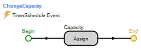
Figure 16.19: Changing the Capacity of the Timer Event
16.4.9 Insert an Assign step that makes the following two assignments (see Figure 16.20). The first assignment will assign GStaTimePeriod the value of zero through eleven by using the Math.Remainder function.259 The next assignment will assign the current capacity of the SrvFirstLineTech Server a value from the table TableSchedule.260 The simulation will start at Run.TimeNow is equal to zero, which is why we added one.

Figure 16.20: Assignments to Perform our Manual WorkSchedule
16.4.10 Return the Facility tab and change the Capacity Type back to “Fixed” since we are performing the manual work schedule.
16.4.11 In order to visually see if our new manual schedule is working, select the SrvFirstLineTech, and from the Animation tab, insert a new Status Label with an expression of CurrentCapacity, as shown in Figure 16.21.
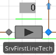
Figure 16.21: Inserting a Status to Watch the Current Capacity
16.4.12 Save and run the model, comparing the results to the previous model.
16.4.12.1 Does the capacity of the server change during each hour’s break?
_______________________________________________
16.4.12.2 Compare the results of the following questions to the previous model.
What is the average customer time in the system and the number of calls still in the system at the end of the simulation?
_______________________________________________
What is the average utilization of the first line and the experienced technicians?
_______________________________________________
What is the average holding time in minutes for both of the two servers’ input buffers?
_______________________________________________
What is the average number of calls waiting in the two server’s input buffer?
_______________________________________________
How many calls balked on average during the 12-hour period, and do you feel the current system is handling enough of the calls?
_______________________________________________
16.4.13 In the assignment, we manually converted the current simulation time into a row index (i.e., GStaTimePeriod), which, if we ran the simulation for 14 hours, would have started over at rows one and two for the 13th and 14th hour. Data Tables in SIMIO can be specified as being Time-Indexed, which allows one to access a column value based on the current simulation time. Select the table properties of the TableSchedule and specify under the Advanced Options that it is Time-Indexed, as shown in Figure 16.22. The starting time will tell SIMIO how to convert the current simulation time into which row, while the Interval Size determines the length of the time bucket to map to each row in the data table.261

Figure 16.22: Making a Data Table Time-Indexed
Two table functions associated with time-indexed data tables can be used to retrieve column values or the current row index, as described in Table 16.4.
| Function | Description |
|---|---|
| TableName.ColumnName.TimeIndexedValue | The TimeIndexedValue will return the value of the column or property that has been specified for the current simulation time (i.e., TimedIndexedValue) |
| TableName.TimeIndexedRow | This function will return the current row index based on the current simulation time. |
16.4.14 From the Processes tab, modify the Assign step by removing the first assignment, which sets the StaTimePeriod and then sets the current capacity to TableSchedule.Capacity.TimeIndexedValue, as seen in Figure 16.23.
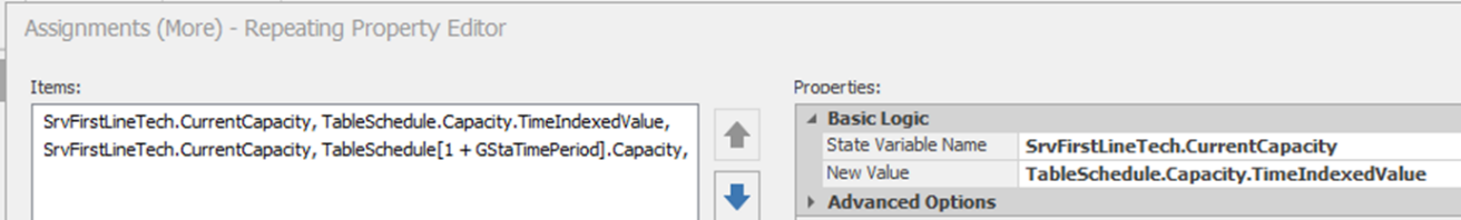
Figure 16.23: Using the TimeIndexedValue Function to Set the Current Capacity
16.4.15 In the Facility window, insert two more status labels with expressions set to TableSchedule.Capacity.TimeIndexedValue and TableSchedule.TimeIndexedRow to see how these values change over time.
16.4.16 Save and run the model, comparing the results to the previous model.
16.4.16.1 Does the capacity of the server change at each hour break in a similar fashion?
_______________________________________________
16.4.16.2 Compare the results of the following questions to the previous model.
_______________________________________________
What is the average customer time in the system and the number of calls still in the system at the end of the simulation?
_______________________________________________
What is the average utilization of the first line and the experienced technicians?
_______________________________________________
What is the average holding time in minutes for both of the two servers’ input buffers?
_______________________________________________
What is the average number of calls waiting in the two servers’ input buffers?
_______________________________________________
How many calls, on average, balked during the 12 hours, and is this a good system now?
_______________________________________________
16.4.17 Now that we have created a manual work schedule that can be optimized to demonstrate the use of time-indexed tables, we will utilize the built-in WorkSchedule. From the Data tab, modify the WorkSchedule to utilize all the time period properties for each of the values, as seen in Figure 16.24.262
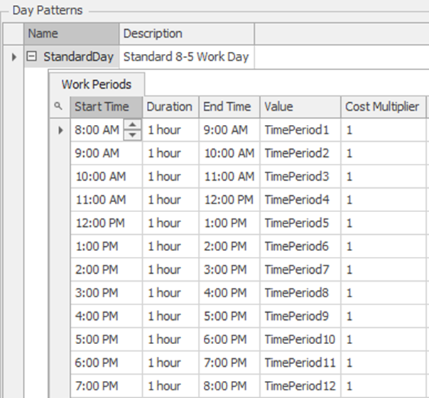
Figure 16.24: Using Properties for the Values of a WorkSchedule
16.5 Using the Financial Costs as the Optimizing Objective
Since the Table to perform the task of developing a manual WorkSchedule has been set up, we can use OptQuest™ to optimize the 12-time period properties. Our goal is now to minimize the costs associated with staffing the call center while balancing our customers’ wait time and the amount of balking and reneging that occurs to reflect customer dissatisfaction. SIMIO introduced ABC costing for many objects under the “Financials“ property section. This cost information can be associated with dynamic (i.e., ModelEntities, Transporters, and Workers) and fixed objects (i.e., Servers, Sinks, Resources, etc.). Therefore, you do not have to capture this information using state variables manually. The following tables explain the financial cost properties of fixed objects (see Table 16.5), vehicle and worker objects (Table 16.6), and model entities (see Table 16.7).
| Property | Sub Property | Description |
|---|---|---|
| Parent Cost Center | The cost center element, which is the cost accrued to this server, is summed up. If the property is left blank, then the costs accrued are rolled up into the parent object containing the server (i.e., the Model). | |
| Capital Cost | The one-time occurrence cost to build this fixed object occurs at the simulation’s beginning. | |
| Buffer Costs (Input, MemberInput, MemberOutput, ParentInput, ParentOutput and Output Buffer) | Cost Per Use | Costs associated with the buffers. This is a one-time use for every entity that enters the buffer regardless of how long they wait in the buffer (i.e., all entities will enter the input and output buffer regardless if they only stay in zero minutes. |
| Holding Cost Rate | This is the cost rate applied per entity based on the amount of time the entity waits in the buffer. | |
| Resource Costs (All fixed objects) | Idle Cost Rate | The cost charged per unit of time for any scheduled capacity of the object that is not utilized. |
| Cost Per Use | This is a one-time use for every time the object is used, regardless of how long the object is used. | |
| Resource Costs | Usage Cost Rate | The cost charged per unit of time for any scheduled capacity of the object that is utilized. |
| Property | Sub Property | Description |
|---|---|---|
| Parent Cost Center | See Table 16.5 for an explanation. | |
| Capital Cost Per Worker/Vehicle | One-time occurrence cost to add this Vehicle or Worker. | |
| Transport Costs | Cost Per Rider | The cost associated with loading/unloading and transporting an entity regardless of ride time. |
| Transport Cost Rate | This is the cost rate applied per entity based on the amount of time the entity waits in the buffer. | |
| Resource Costs | Idle Cost Rate | The cost charged per unit of time for any scheduled capacity of the server that is not utilized. |
| Cost Per Use | This is a one-time use for every time the object is used, regardless of how long the object is used. | |
| Usage Cost Rate | The cost charged per unit of time for any scheduled capacity of the Vehicle/Worker that is utilized. |
| Property | Description |
|---|---|
| Initial Cost | The initial cost for the creation of the ModelEntity. |
| Initial Cost Rate | The cost charged per unit of time for any scheduled capacity of the server that is not utilized. |
16.5.1 Select the SrvFirstLineTech Server and expand the “Financials” property category. The first-line technicians receive $25 per hour regardless of whether they are helping a customer or not. Therefore, set the Idle and Usage Cost Rate properties to “25 as shown in Figure 16.25. Owing to the trunk line rentals, there is a fixed cost (i.e., $10) regardless of usage as well as a $5 per hour per call usage rate that needs to be specified. We will leave the Parent Cost Center blank to utilize the Model’s cost center.263
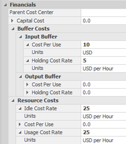
Figure 16.25: Specifying Cost Information on the Server
16.5.2 Since our cost information is set up, we now need to optimize the number of technicians by minimizing the total costs associated with the system while balancing the number of unhappy customers. Create a “New Experiment” named Optimization.
16.5.3 Add the following three responses to the experiment, which will determine the total cost of the system and keep track of the number of people who balk and renege.
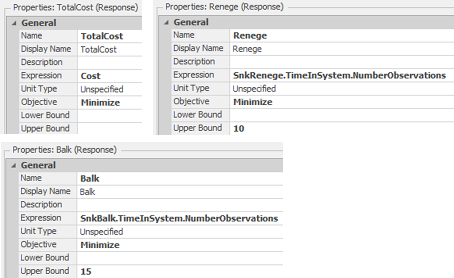
Figure 16.26: Add the Three Responses of Cost, Number Reneging, and Number Balking
16.5.4 Like many problems, this is a multi-objective problem where the objectives often conflict (i.e., on the one hand, minimizing the number of technicians would minimize cost, while customers would like the maximum allowed at each period to minimize their wait time). As was done previously, we can convert the multi-objective by combining the objectives in a weighted fashion, which generally is not a bad idea.264 Instead, we will utilize thresholds or bounds on the number of balking and reneging. Having 25 people balk or renege represents, on average, approximately 3% of the callers that are seen in the day, which is what management feels is adequate for customer satisfaction. We set the upper bounds of 15 and 10 for the number of people who are acceptable to balk and renege, respectively, as seen in Figure 16.26.
16.5.5 From the Add-Ins section of the new experiment, select the OptQuest for SIMIO add-in. Next, for each of the 12 Control variables, specify the Minimum Value to be “1”, the Maximum Value to be “20”, and the Increment property value to be “1”. Properties of the model become Control variables automatically.
16.5.6 Specify the TotalCost response as the Primary Response, as seen in Figure 16.27. Also, set the OptQuest™ parameter values based on the figure. We will need to run this optimization longer based on the number of variables and threshold constraints.
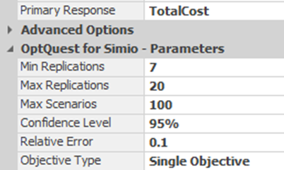
Figure 16.27: OptQuest™ Parameter Values
16.5.8 Once the optimization is complete, filter the scenarios so that only the ones that are checked are present, representing the scenarios that meet the number of balking and reneging thresholds.265 Next, sort the total cost column in ascending order. At this point, you should run the K-N selection algorithm on the top 20 or so scenarios to determine the best since only seven replications were used. Use a $100 indifference zone.
16.5.8.1 What did you get for the total cost of the best system?
_______________________________________________
16.5.9 The optimization has determined that more than 140 technician hours are needed based on costs. However, management only has access to 135 total hours. Add a constraint, which is a constraint on the decision control variables that utilizes the following expression, as shown in Figure 16.28.
TimePeriod1 + TimePeriod2 + TimePeriod3 + TimePeriod4 + TimePeriod5 + TimePeriod6 + TimePeriod7 + TimePeriod8 + TimePeriod9 + TimePeriod10 + TimePeriod11 + TimePeriod12
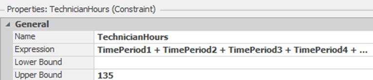
Figure 16.28: Specifying Control Variable Constraint
16.5.11 Once the optimization is complete, filter the scenarios so that only the ones that are checked are present, representing the scenarios that meet the number of balking and reneging thresholds. Next, sort the total cost column in ascending order.
16.5.12 Next, run the KN Select Best Scenario algorithm with an indifference zone of $10 on the feasible solutions.
16.5.14 Recall that the KN selection algorithm does not consider constraints on the non-primary objectives. Select the minimum one that meets the two objective thresholds.
16.6 Commentary
- In this chapter, the Execute step was used to create a new Token that worked independently of the original Token. An additional modeling concept can cause the same phenomena to occur. The Exited add-on process triggers for objects can work in a similar fashion. The Exited add-on process triggers are executed when the trailing edge of the ModelEntity has exited the node, link, station, or object, depending on the trigger. Many people do not realize that the logic in these add-on processes runs in parallel while the entity continues to the link, station, etc. To illustrate this fact, you can clear the Entered Add-on process trigger for the SrvFirstLineTech and then select the Input node of the server. Set the Exited add-on-process trigger of the Input@SrvFirstLineTech BasicNode to be the RenegeProcess and rerun the model, comparing the results to the previous section.
- All of the SIMIO objects that Input and/or Output buffer stations have built-in Balking and Reneging options, which can handle very simple cases.
- More complicated reneging processes can also be utilized. For example, every five minutes, you are told how many people are still in line, and the person could make a probabilistic decision based on some behavior (i.e., number of people and how long they have already been waiting), as seen in Figure 16.29. In this example, if they search for the entity in the queue as before, it will decide to renege or not. If they decide not to renege (i.e., “True” path), it loops back and delays for another five minutes. The same remove and transfer is utilized if the caller decides to renege. The looping will continue until the caller no longer remains in the queue or reneges and leaves the system.
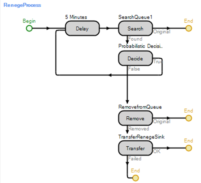
Figure 16.29: Reneging Process that Checks Every Five Minutes
We could have modeled the whole 24 hours with the other intervals values being set at zero. However, we changed the run length of our simulation to only be 12 hours.↩︎
We find it easier to set the Start Time and then the duration which will automatically set the End Time.↩︎
There are many ways to model the balking procedure. One could use the balking parameters under the Input Buffer Logic in the Server. Or, one could add three TransferNodes with the first transfer based on the number in the queue by setting the link weights (i.e., <= 10 , > 10 && <=20, >20 && <= 30, and > 30). Then set the appropriate link weights based on the percentages from the Transfernodes to the SrvFirstLineTech or the SnkBalk.↩︎
It is not strictly necessary to include the values for 0 and for 200, since the table assumes the last value if the lookup is outside the range of the table – a value less than or equal to 10 will be 0 and values equal to or greater than 31 will be 0.5.↩︎
Otherwise, the Server will be executing the process without the ModelEntity and it will crash when performing the Search step.↩︎
Typically it is a good idea to create properties for values rather than hardcoding values which makes it easier to change later.↩︎
See Chapter 13 for a discussion on using the Search step to look through collections.↩︎
Recall the Remove step can be used to remove entities from storage and allocation queues only.↩︎
Create one property with the correct category, a name of TimePeriod, and then copy it changing the default value to the correct values.↩︎
The easiest way is to utilize Excel to create the 12 rows. First, add TimePeriod1 and TimePeriod2 into two different cells. Then select both of these cells and drag down letting excel create the other ten rows. Then copy and paste the Excel table into the TableSchedule.↩︎
In this example, the remainder function takes care of the fact that Run.TimeNow will reach 12 and therefore the remainder will be zero and start over. If you are running 24 hours for more than one day then using Math.Remainder(StaTimePeriod, 24) is the way to get the correct time period for each day.↩︎
Row indexes start at one and therefore we need to add one to the StaTimePeriod to get the correct period.↩︎
SIMIO is internally doing what we did to calculate the row index.↩︎
The easiest way to set the values is to copy them again from Excel which can be used to create the column.↩︎
A Cost Center element can be specified to have the cost summed up. These cost centers can be specified in a hierarchical fashion (i.e., several object roll up to one center for total costing (e.g., department costing), several centers can roll up to higher level centers (e.g., departments to a plant, plants to organizations, etc.). You can also use Assign steps to assign costs to centers dynamically.↩︎
We could arbitrarily put a large cost on the input buffers of both the balk and renege Sinks to try to force the system to minimize the number of balking and reneging that occurs. However, determining the right value of the cost can be difficult.↩︎
Select the filter option in the column heading row above the check boxes.↩︎