Simulation Modeling with Simio - 6th Edition
Chapter
10
Inventories, Supply Chains, and Optimization
Many industries/companies are facing many challenges in their effort to compete in the global marketplace. Demand variations, long lead times, and raw material supply fluctuations can result in excessive finished goods inventory and/or poor customer service levels. Many companies with longer lead times are forced into a make-to-stock policy to respond to customer demands and quickly maintain market share. Too much inventory will create higher costs and may lead to product obsolescence or spoilage, while too little inventory may cause stockouts and lower customer service levels. Therefore, designing and optimizing a company’s supply chain has become a priority as it is becoming a necessity for the survival of many companies. The main objective of any supply chain is to supply the customer with a product when the customer wants it and at a price that maximizes profit. To achieve both objectives, a balance must be struck between carrying sufficient inventories to meet demand and not so much negatively impacting profitability.
10.1 Building a Simple Supply Chain
Figure 10.1 shows a very simple three-tier supply chain where customers arrive at a store, which could be a collection of stores to purchase a product. The stores place orders at the manufacturer’s DC (Distribution Center), which will supply the product if it is in stock. The DC uses an inventory model to determine reorder policies for the supplier, which is assumed to have a raw material source. It takes between three to six days to truck the product from the supplier to the manufacturer.

Figure 10.1: Simple Three-Tier Supply Chain
The goal is to track the DC’s average inventory and service level/fill rate over a year. Therefore, the store customers will not be part of the current model since the manufacturer is interested in determining the reorder point and reorder quantity. The store reorders daily from the DC, and the DC utilizes a (s, S) periodic review inventory model, as seen in Figure 10.2. In this model, the inventory is reviewed at every fixed time interval, called the period. An amount s is the re-order point, a quantity below which triggers a re-order. The quantity S is determined as the quantity needed after inventory is re-ordered (an order-up-to amount).
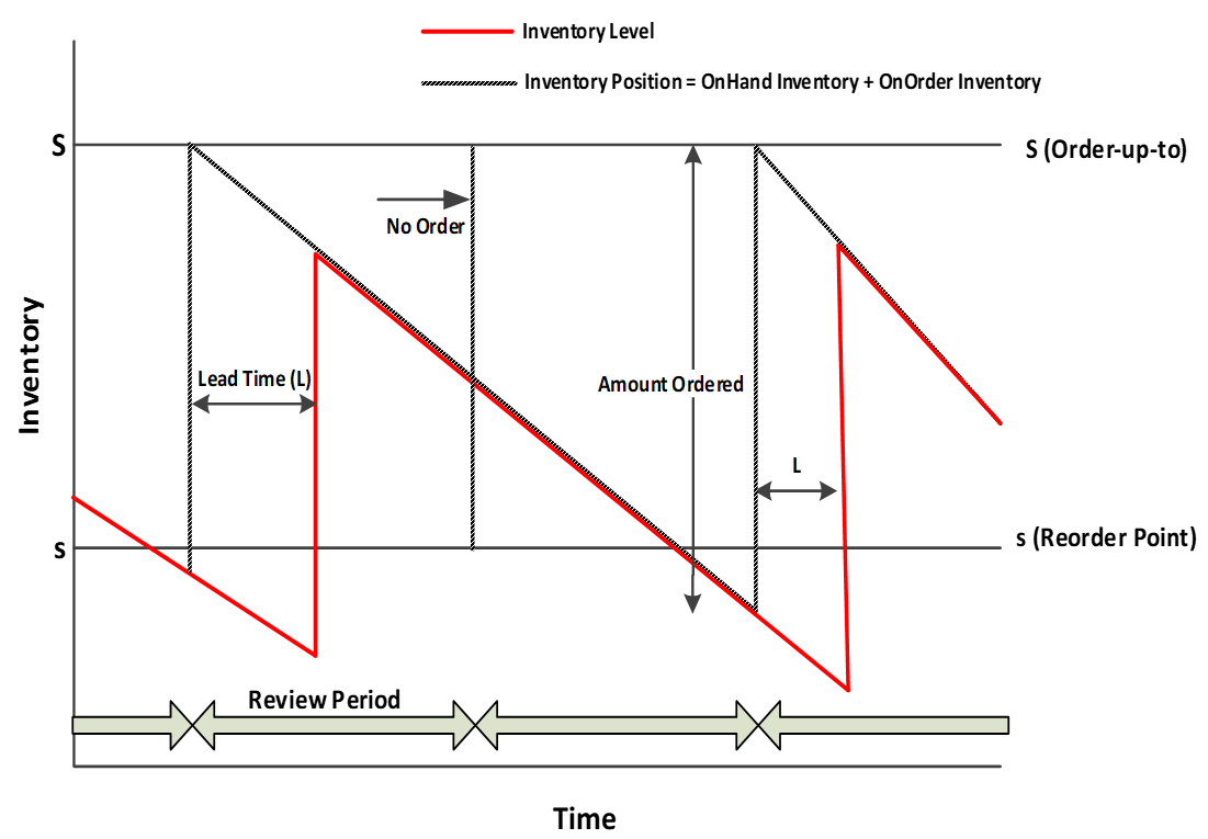
Figure 10.2: (s, S) Inventory Policy
10.1.1 Create a new model with two separate systems, as seen in Figure 10.3.
- The first system will model the ordering portion of the supply chain (i.e., orders from the store placed at the DC will need to be processed). Insert a Source named SrcOrders, a Server named SrvOrderProcessing, and a Sink named SnkStore. A new ModelEntity named EntOrders should also be inserted, making sure the SrcOrders creates these EntOrders. Use connectors to link the objects together, modeling Electronic Data Interchange transactions between the stores and the DC.
- The second system will model the flow of products from the back of the chain to the front of the supply chain used to replenish the inventory in the manufacturer’s DC. Insert two Servers named SrvSupplier and SrvDC, a Sink named SnkDCInventory, and another ModelEntity named EntReplenishments. Connect the SrvSupplier and SrvDC via a Time Path that uniformly takes between one and two days. Use a connector from the SrvDC to the SnkDCInventory since the model is really only concerned with the DC.

Figure 10.3: SIMIO model of the Three Tier Supply Chain Re-ordering Process
10.1.2 Since we will not model every item in the inventory system as a separate entity, add a Discrete Integer State variable named EStaOrderAmt to the ModelEntity129 to represent the quantity of products for each store order or replenishment re-order.
10.1.3 For the Ordering process, set the following information.
- Change the SrcOrders to have one order arrive daily.
- The amount of each order that arrives daily from the store is Poisson distributed with a mean of 40. As seen in Figure 10.4, use the State Assignments→Before Exiting property of the source to set the ModelEntity.EStaOrderAmt to a Random.Poisson(40) .

Figure 10.4: Specifying the Order Amount of each Order
10.1.4 Next, under the Definitions→Properties of the model, insert four Expression Standard Properties named InitialInventory, ReorderPoint, OrderUptoQty, and ReviewPeriod. These should all be placed in the “Inventory” Category.130
| Property | Default Value | Category | Unit Type | Description |
|---|---|---|---|---|
| InitialInventory | 700 | Inventory | Unspecified | The initial inventory at the start of the simulation. |
| ReorderPoint | 300 | Inventory | Unspecified | Determines the point to re-order. |
| OrderUptoQty | 700 | Inventory | Unspecified | The maximum inventory to order up to quantity. |
| ReviewPeriod | 5 | Inventory | Time (Days) | The periodic review period |
10.1.5 In the Model, insert a discrete integer state variable named GStaInventory, which will represent the current inventory amount (“OnHand”) of the product at the DC, and another one named GStaOnOrder (i.e., work in process), which represents the total amount the DC has currently ordered (“OnOrder”) from the supplier. The Initial State Value property should be 0 for both the GStaInventory and GStaOnOrder variables, respectively.
10.1.6 Next, we need to insert several Elements into the model, as seen in Figure 10.5.
- Insert a Tally Statistic named TallyStatFR to track the fill rate (i.e., service level performance).
- Insert a StateStatistic named StateStatInv to track the inventory level performance. Specify the State Variable Name property as the GStaInventory variable.
- Insert a Timer named TimerReview to model the review period. The DC currently reviews its inventory level every five days and should utilize the ReviewPeriod property (see Figure 10.5).
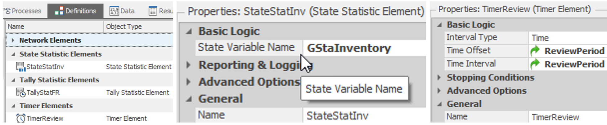
Figure 10.5: Setting up the Statistics and Periodic Review Timer
10.1.7 Change the Processing Time property of SrvOrderProcessing such that orders take ½ a day to be processed before an attempt is made to fill the order with the available inventory.
10.1.8 The supplier will take between 10 and 20 minutes, with the most likely time being 15 minutes, to process each product. Therefore, the total processing time for one order would be the sum of several triangular distributions (i.e., an order amount).131 Again, the Math.SumofSamples function handles the processing of the batch correctly by sampling from the distribution the appropriate number of times. For the SrvSupplier, specify the Processing Time property to Math.SumOfSamples(Random. Triangular(10,15,20), ModelEntity.EstaOrderAmt) uses the order amount to determine the number of triangular distributions to sample and sum, as seen in Figure 10.6.
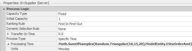
Figure 10.6: Specifying the Operation Quantity and Batch Size for Processing of an Order
10.1.9 Once the product arrives at the DC, the entire lot must be individually packaged before it is available to satisfy the store's demands. Therefore, set the SrvDC’s Processing Time property to Math.SumOfSamples(Random.Pert(1,2,5), ModelEntity.EstaOrderAmt) in minutes.
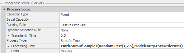
Figure 10.7: Setting up the DC Server Properties to Process the Batch
10.2 Processing Orders in the Supply Chain System
Recall that the initial inventory level property (i.e., InitialInventory) was created to allow for changing the initial condition at the model level. ### Since state variable default values cannot be reference properties, the state variable GStaInventory needs to be initialized at the beginning of the simulation via the OnRunInitialized process of the model. Insert this process by selecting it via the Processes→Select Process→OnRunInitialized dropdown menu. Insert an Assign step that assigns the GStaInventory state variable the InitialInventory value, as seen in Figure 10.8.
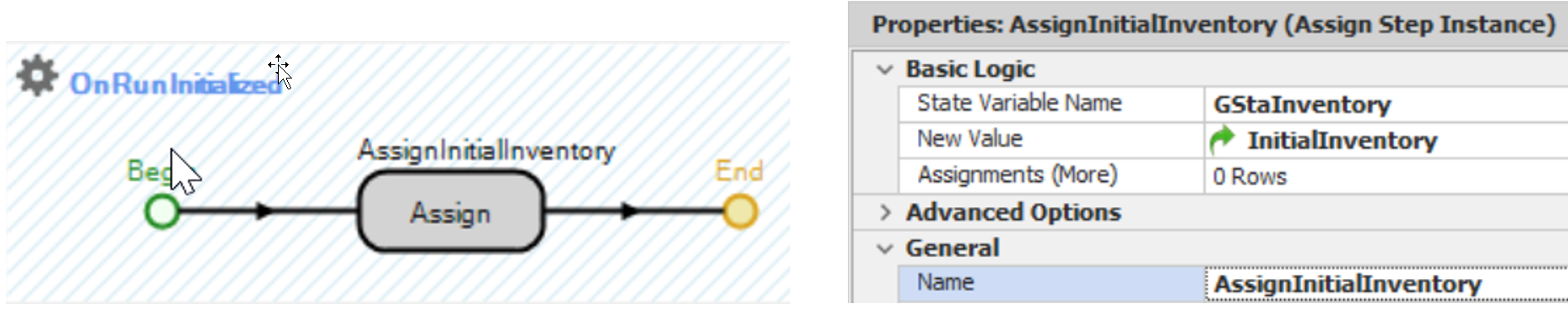
Figure 10.8: Assigning the Initial Inventory Level
10.2.1 EntOrders must be filled based on the current inventory position when they arrive at the DC and have been processed.132 Therefore, insert a new “After Processing” add-on process trigger for the SrvOrderProcessing Server to handle the behavior (i.e., update the current inventory position and service level).
- Add a Tally step to update the Tally Statistic TallyStatFR with the value equal to Math.Min(1,GStaInventory/ModelEntity.EStaOrderAmt).133
- Next, insert an Assign step that will update the current GStaInventory level by subtracting the EStaOrderAmt of the particular order from the inventory on hand. However, if the GStaInventory level is less than the order amount, it would be negative. Since we are not allowing backorders, we should set the level to the following expression, as seen in Figure 10.10.
- Math.Max(0,GStaInventory-ModelEntity.EStaOrderAmt)
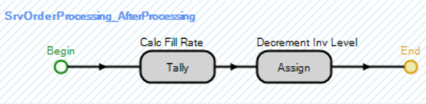
Figure 10.9: Process to Fill Demands from the Stores
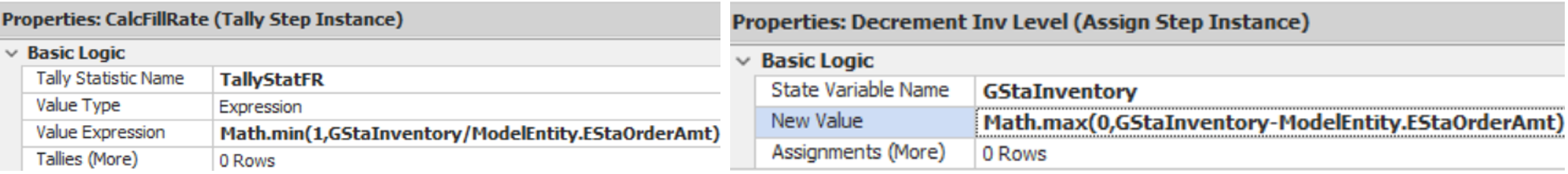
Figure 10.10: Properties of the Steps
10.2.2 To track the information while the simulation is running, insert a “Status Table” from the “Animation” tab, as seen in Figure 10.12, to track the current average inventory and service levels. To populate the “Status Table,” insert a Data table named TableLabels with a String Property column named Type and an Expression Property column named Value. The first column of labels is the description, while the second column uses the expressions GStaInventory, GStaOnOrder, GStaInventory+GStaOnOrder, StateStatInv.Average, and TallyStatFR.Average.134
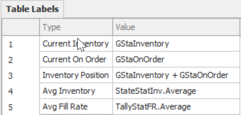
Figure 10.11: Table to Be Used with a Status a Status Table
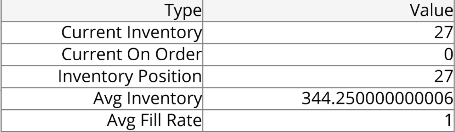
Figure 10.12: Status Table to Show Current Inventory Level and Average Inventory and Fill Rate
10.2.3 From the “Animation” tab, insert a new Status Plot that will track the current onhand inventory level, the replenishment on order, and the inventory position representing the onhand plus the on order. Using the Additional Expression property, add three items to the plot, as seen in Figure 10.13, and make the “Time Range” equal to “1” week.

Figure 10.13: Setting up the Status Plot to Track Inventory and On Order Amounts
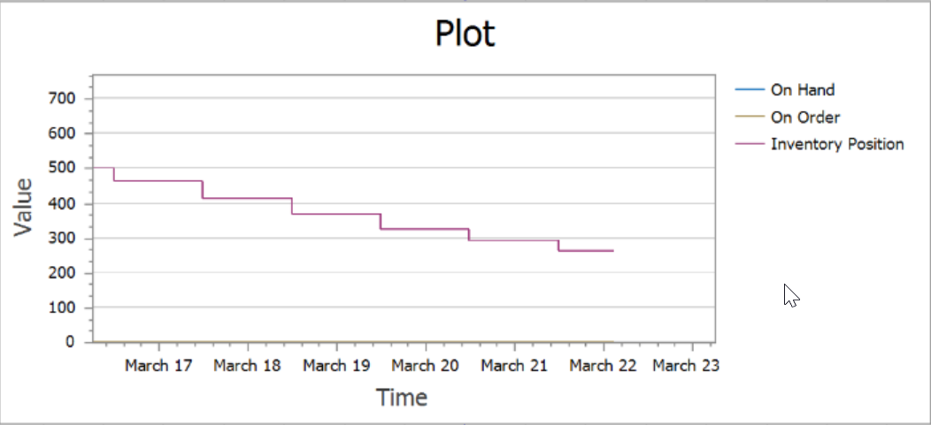
Figure 10.14: Status Plot Showing Inventory Positions
10.3 Creating the Replenishment Part of the Supply Chain System
The previous section handled demand orders from the stores, but once the inventory was depleted, there was no inventory replenishment. Hence, the service level was abysmal. The timer was set up to fire every five days. At that time, if the current inventory is below the re-order point, a replenishment order should be sent to the supplier based on the order-up-to quantity, the current inventory level, and the current number of outstanding orders (i.e., On Order). Recall that the “inventory position” is defined as the current inventory on hand plus the inventory represented in outstanding orders.
10.3.1 Create some statistics on the replenishment procedure:
- Insert a State Statistic, called StateStatOnOrder, to keep track of the amount of inventory on order over time. This statistic should reference the GStaOnOrder state variable.
- Insert a Tally Statistic, called TallyStatAmtOrdered, to record the amount ordered from the supplier.
- Add StateStatOnOrder.Average and TallyStatAmtOrdered.Average to the TableLabels to update the “Status Table.”
10.3.2 Set up the periodic review to happen by creating a process to respond to the timer TimerReview. From the “Processes” tab, insert a new process named InventoryReview. Set the Triggering Event property to react to the TimerReview.Event, which causes the process to be executed every time the timer event fires, as seen in Figure 10.15.
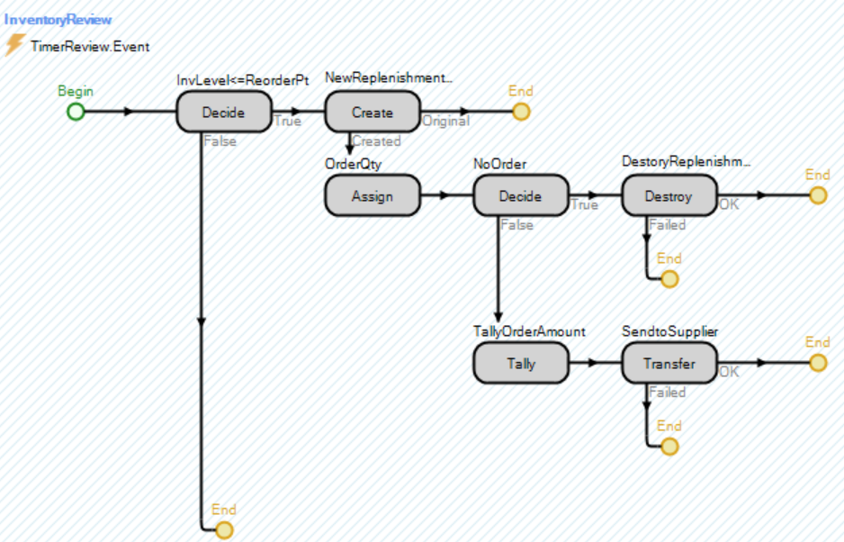
Figure 10.15: Process to Re-order
- Insert a Decide step that uses a “ConditionBased” check to see if the current inventory is less than the re-order point (i.e., GStaInventory <= ReorderPoint).
- If a new replenishment (i.e., “True” branch) is needed, use the Create135 step to create a new EntReplenishments entity, as seen in Figure 10.16.
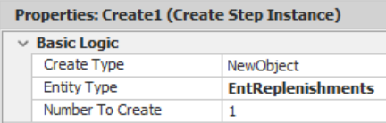
Figure 10.16: Creating a New ReOrder to Send the Supplier
- For the newly created EntReplenishments, use an Assign step to assign the order amount and then increase the StaOnOrder value based on the order amount.
| State Variable | New Value |
|---|---|
| ModelEntity.EStaOrderAmt | Math.Max(0,OrderUptoQty-GStaInventory-GStaOnOrder) |
| GStaOnOrder | GStaOnOrder + ModelEntity.EStaOrderAmt |
- In the second Decide step, determine if the EStaOrderAmt is zero (i.e., ModelEntity.EStaOrderAmt==0). Namely, no replenishment order is needed (an assumption here is that there are never any zero quantity replenishment orders)
- If no replenishment order is needed, then the replenishment order entity is destroyed using the Destroy step.
- Otherwise, the amount of the replenishment order (ModelEntity.EStaOrderAmt) is tallied via the TallyStatAmtOrdered.
- Once the EntReplenishment has been tallied, it must be sent to the supplier using a Transfer step to move it from “FreeSpace” to the Input node of the WrkSupplier.136
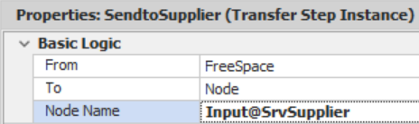
Figure 10.17: Setting up the Status Plot to Track Inventory and On Order Amounts
10.3.3 When the products arrive back at the DC and have been packaged, the GStaInventory variable must be increased by the order amount. At the same time, the same value reduces the GStaOnOrder variable. Insert the “AfterProcessing” add-on process trigger for the SrvDC, as seen in Figure 10.18. Insert an Assign step that updates the values in Table 10.3.

Figure 10.18: Setting up the Status Plot to Track Inventory and On Order Amounts
| State Variable | New Value |
|---|---|
| GStaInventory | GStaInventory + ModelEntity.EStaOrderAmt |
| GStaOnOrder | GStaOnOrder - ModelEntity.EStaOrderAmt |
10.3.4 Save and run the model (you may need to fast-forward the simulation) for 26 weeks.
10.3.5 You may notice that the status table displays as many significant digits as possible for the average inventory and the servicelevel/fill rate. SIMIO exposes many of the .Net string manipulation functions. For example, the String.Format function can be used to format the output.137 Replace the two average and service-level status labels with the ones in Table 10.4.
| Status Label | Expression |
|---|---|
| Average Inventory | string.format(“{0:0.##}”,StateStatInv.Average |
| Average OnOrder | string.format(“{0:0.##}”,StateStatOnOrder.Average) |
| Average Fill Rate | string.format(“{0:0.00%}”,TallyStatFR.Average) |
| Average Replenishment Qty | string.format(“{0:0.##}”,TallyStatAmtOrdered.Average) |
10.4 Using an Experiment to Determine the Best Values
Simulation is often used to improve a system. Can we find a better order-up-to-quantity and re-order point that improves the system's overall performance? Can SIMIO provide help with this kind of question? Or can SIMIO help in searching for an improved system? The answer is yes to all these questions.
10.4.1 From the Project Home→Create section, insert a new “Experiment” named FirstExperiment. This will create a new experiment window and automatically create the first scenario, which is the base model, as seen in Figure 10.19. SIMIO automatically added the four properties as control variables.138
10.4.2 Insert eight more scenarios by clicking the little box in the last row. This will copy all of the parameters from the base case. Then, change re-order points and order up to quantities to do a full factorial experiment of the three re-order points (200, 300, and 400) and order up to quantity (600, 700, 800), as seen in Figure 10.19. Change the names of the scenarios so they can be interpreted.
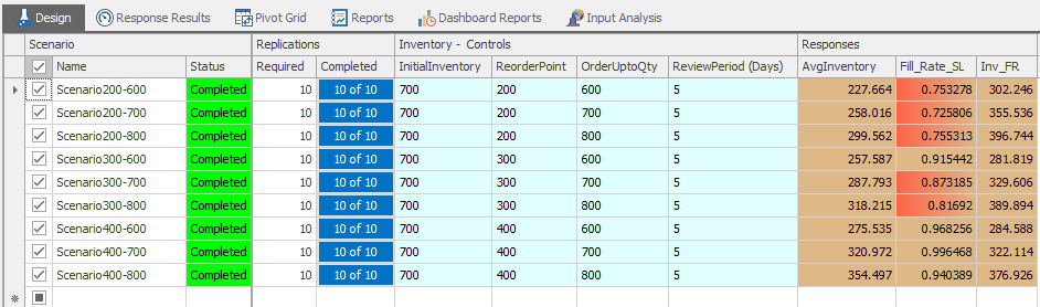
Figure 10.19: First Experiment Trying Different Re-order Points and Order Up to Quantities
10.4.4 Figure 10.20 shows the basic experiment parameters, where you can define the warm-up period and the default number of replications that all scenarios will run. For the SMORE plots and optimization, the confidence interval and upper and lower percentiles are displayed. Also, you need to define the primary response that the ranking and selection will use and Optquest™ add-ins (see the next sections).
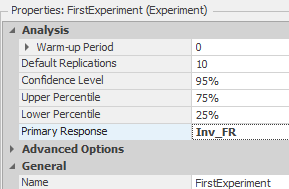
Figure 10.20: Setting up the Experiment Parameters
10.5 Using SMORE Plots to Determine the Best Values
In the previous section, we just used the average of the ten replications to assist you in choosing the best selection. The difficulty is that the variability of the system is not accounted for when selecting the best scenario. “SIMIO Measure of Risk & Error” (SMORE) plots offer the ability to see the variability and confidence intervals. They show the significant percentiles (median or 50th percentile, lower chosen percentile, and upper chosen percentile), mean, and confidence intervals for the mean and the percentiles.
10.5.1 Select the “Response Results” tab from the previously run model to see the SMORE plots. The primary response (Inv_FR) will be displayed by default, but the other response can be selected from the dropdown, as seen in Figure 10.21. Quickly, we can see from the “AvgInventory” response that Scenario200-600 seems to be the best, and its variation is clear from the other plots. Scenario 300-600 appears to be the second best; however, its variation overlaps with Scenario 200-700. However, when looking at the service level with the limits turned on, only Scenario300-600, Scenario400-600, Scenario400-700, and Scenario400-800 meet the 90% service level limit, with the Scenario400-700 seeming statistically the best. Considering the two plots together, Scenerio300-600 appears to be the better choice.
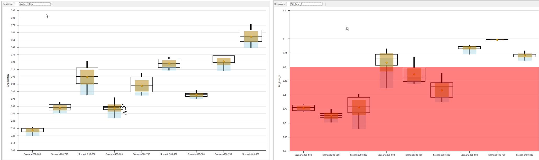
Figure 10.21: SMORE Plots of the Average Inventory and Average Service Level
10.5.2 Looking at the Primary Response (“Inv_FR”) SMORE Plot in Figure 10.22, Scenario 300-600 appears to be the best, based on the combined response. However, its confidence interval does overlap with Scenario400-600.140
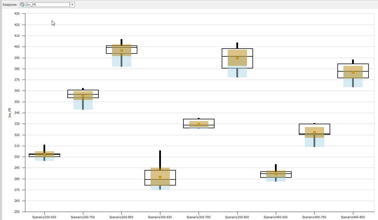
Figure 10.22: SMORE Plots of the Combined Inventory/Service Level Response
10.5.3 By clicking the “Subset Selection” option in the “Analysis” section of the ribbon in the “Design” tab, you can see the choices made by a series of algorithms within SIMIO. Scenarios for each response are divided into the “best possible group” and the “rejects group”, as shown in Figure 10.23.
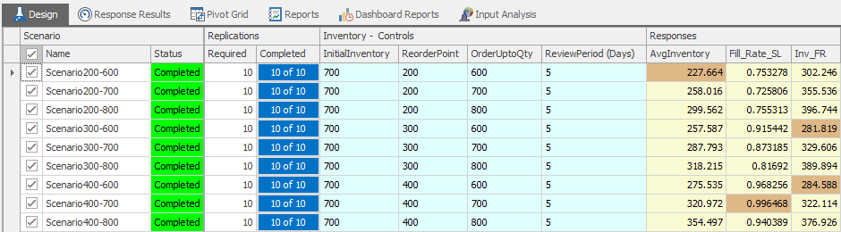
Figure 10.23: Using Subset Selection
While the best possible group may consist of scenarios that cannot be proven statistically different from each other, it can be shown that the best possible group scenarios will be statistically better than the rejected group (shown in muted color). You can see that the two best scenarios on response Inv_FR are not statistically different.
10.6 Using Ranking and Selection to Determine the Best Scenario
The analysis is quite simple (focused on only two variables within the model), and ten replications seemed enough to choose the best. However, using the SMORE plots still requires judgment or visual identification. Ranking and selection methods allow you to determine statistically which scenario is the best. One of the advantages of SIMIO is the two built-in state-of-the-art ranking and selection methods. One is based on research by Kim and Nelson (called “KN”),141 and the other one is by Ma and Henderson (called GSP).142 The GSP method may improve performance when doing large-scale models that require many scenarios in a parallel processing environment.
10.6.2 Next, choose “Select Best Scenario using KN” from the Design→Add-Ins section, as shown in Figure 10.24.

Figure 10.24: Selecting the KN Algorithm Add-in
10.6.3 This will add the KN algorithm to the experiment (see Figure 10.23) and give you additional properties. Set the Indifference Zone property to five, which stipulates that one solution can be determined better than another only if the two solutions differ by more than five. Since the ranking and selection scheme will change the number of replications during its execution, the Replication Limit property specifies the maximum number that can be run.
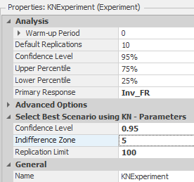
Figure 10.25: Setting up the KN Parameters
10.6.4 Set the number of “Required” replications (under the Replications category) to one each, make sure that each scenario is “checked” (in the left column), and “Reset” the experiment.
10.6.5 Run the experiment and notice that the number of replications required for each scenario increases to ten. The KN algorithm requires at least ten replications to detect a difference among scenarios reliably.
10.6.6 The KN algorithm has selected Scenario 300-600 as the best (the only one checked), as seen in Figure 10.26. Figure 1.23 shows that Scenario 300-600 and Scenario 400-600 were statistically identical. KN required additional replications on those two scenarios to determine which was statistically better on the indifference zone of five.

Figure 10.26: : Results of running the KN
10.6.8 Reset the experiment, select all the scenarios again, and change the required to 10. Change the indifference zone to one and rerun the experiment to see the impact. Figure 10.27 displays the algorithm's results. You can see two additional scenarios needed to be run for more than the default ten replications, and the two very close scenarios had to be run 86 times to distinguish them with an indifference zone of “1.”
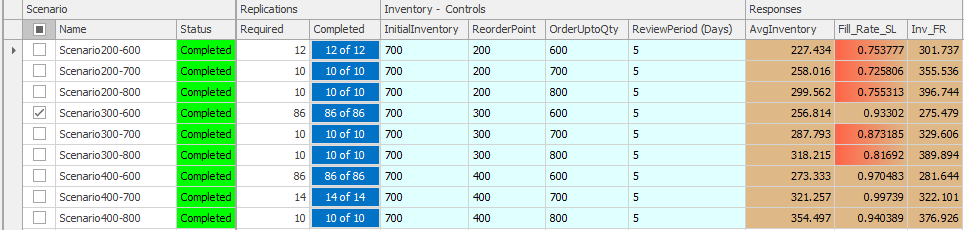
Figure 10.27: Running the KN Algorithm with an Indifference Zone of ‘1’
10.7 Using OptQuest™ to Optimize the Parameters
The KN algorithm used in the previous section determined the optimal scenario from a fixed set of user-defined scenarios. SIMIO has an add-in optimizer, OptQuest™, that can perform traditional optimization by trying other values for the decision variables not specified. It will also allow constraints on the decision variables and output responses, which the KN and GSP cannot.143 ### Save the current model and, duplicate the FirstExperiment and then rename the new experiment OptQuestExperiment. ### Use the “Clear” button to remove the Select Best Scenario add-in and then select the OptQuest for SIMIO add-in if you duplicated the KNExperiment instead. ### Since the optimizer will try different values for our control (decision) variables, we must define their valid ranges. Select appropriate ranges and increment values to speed up the convergence and potentially the solution quality. Select each control variable and set their values according to Figure 10.28. As you can see, the Initial Inventory is not included in the optimization. An increment value of 25 was chosen for the other two variables to allow the algorithm to select values only in increments of 25.144
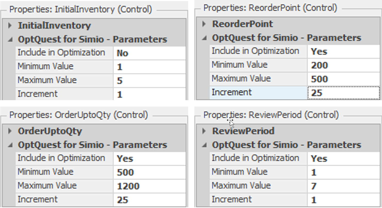
Figure 10.28: Setting the Lower and Upper Bounds on the Decision Variables
10.7.1 Next, choose the “OptQuest™ for SIMIO” from the Design→Add-Ins section to insert the optimization algorithm. It will add a setup section in the Experiment properties, as seen in Figure 10.29. The algorithm uses a confidence level to distinguish between solutions. The relative error percentage of the confidence level is expressed as a percent of the mean. Notice that a range of replications is specified, and a maximum number of scenarios is specified. These will limit the time OptQuest will spend computationally in the simulations and search for a better solution.
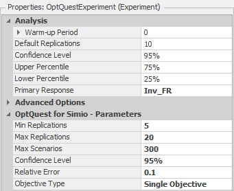
Figure 10.29: SOptQuest Parameters
10.7.2 Save and run the optimization algorithm. Notice how it tries several different variable values of the controls. As specified in the Max Scenarios property, it will create a maximum of 100 scenarios or decision points.
10.7.3 Notice only feasible scenarios with respect to constraints on the responses (i.e., service level greater than 90%) are checked. Click on the little funnel ( ) in the upper right corner of the Fill_Rate_SL response and choose the [Custom] filter option. Set up the filter to only allow feasible scenarios to be visible, as seen in Figure 10.30. Then, sort the scenarios by the Inv_FR column in ascending order to see those with minimum Inv_FR ratios by right-clicking on the column heading.
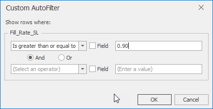
Figure 10.30: Filtering only Solutions that meet the Threshold of 90% Service Level
10.7.6 To see that one is better than the others, examine the Response Chart for the one scenario KN selected, as seen in Figure 10.28. Note that you must “check” the alternative scenarios to see them in the Response Chart. In our example, Scenario 052 (i.e., 300 re-order points and 550 (order-up-to quantity)) was deemed to be the best, with one as the indifference zone.
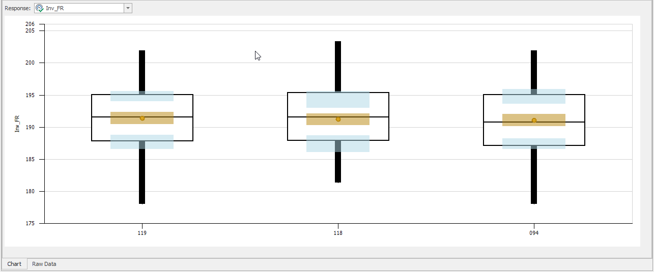
Figure 10.31: Viewing the Best Scenarios Indifference Zone of ‘5’
10.8 Multi-objective and Additional Constraints using OptQuest™
While the KN selection algorithm can statistically determine which scenario is the best, it cannot consider constraints on the responses. Constraints on the control variables should be handled since the scenarios selected should be feasible. Unfortunately, many problems often have multiple conflicting objectives, and it is rare for a single point to optimize all the objectives. Figure 10.32 depicts the efficiency frontier of a problem that optimizes both service level and inventory level at the same time. The frontier represents all non-dominated points that a decision-maker could choose. From the figure, the inventory level could be reduced by half if they were willing to go from 98% service level to around 90% service level.
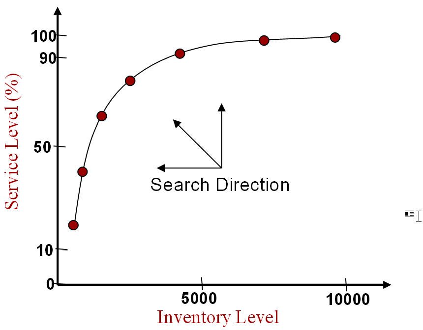
Figure 10.32: Efficiency Frontier
10.8.1 Finding the frontier is very difficult. To help alleviate the problem, many people try to convert the multi-objective problem into a single objective (g(x)) problem. The most common way and easiest way is to aggregate the objectives into a single objective by summing up the weighted objectives (.e., \(g(x) = \ \sum_{i = 1}^{k}{w_{i}f_{i}(x)}\)). The decision maker can determine the importance of each objective by choosing the weights accordingly. SIMIO can automatically create the combined function by specifying the appropriate weights of the responses and choosing the Multi-Objective Weighted value as the Objective Type property of the Experiment, as seen in Figure 10.33.
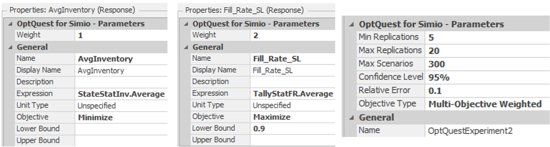
Figure 10.33: Using the Multi-Objective Aggregate Optimization Method
10.8.2 In this example, the decision maker puts twice as much importance on service level as on inventory. The difficulty with this multi-objective approach is scaling the weights to find solutions. In this example, inventory is in the hundreds while service level is less than one. In many cases, the optimization algorithm will only optimize the dominant objective. While this may be a convenient method, one can accomplish the same by creating an aggregate response and specifying the expression as StateStatInv.Average + 2 * TallyStatSL.Average. To avoid the scaling problem (i.e., 100s vs percentages), we created an aggregate response that was minimized by taking the inventory level divided by the service level to try to force the algorithm to minimize the inventory while maximizing the service level.
The other way is to optimize one primary objective (e.g., average inventory) while setting thresholds (i.e., lower and upper bounds) on the other objectives (e.g., the lower bound of 0.90 on service level), which would create one point on the frontier which we did in the previous section. There are two categories of constraints in the OptQuest for SIMIO: constraints on the controls (inputs) and constraints on the responses (outputs).
Suppose we consider a slightly different optimization problem, namely minimizing the average inventory level while keeping the service level above 95%. We can write this more formally using the following equations. Of the three constraints, the last two are simply bounds on the controls. The first constraint restricts the simulation's response (i.e., Fill Rate).
Minimize: AvgInventory
Subject to: Fill Rate >= .95
200 <= ReorderPoint <= 500
500 <= Order UpToQty <= 1200
10.8.3 Select the OptQuestExperiment2 and change the primary objective to be the AvgInventory response and Objective Type to “Single Objective” under the experiment properties.145
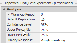
Figure 10.34: Change the Primary Response of the Experiment Properties
10.8.5 Sort the scenarios in the average inventory column in ascending order to see those with minimum average inventory, and filter the service levels to display only feasible solutions.
10.8.6 All of the previous methods made the decision before the search(i.e., the modeler decided which point on the Pareto frontier to generate). OptQuest can also discover the efficiency frontier. Duplicate the OptQuestExperiment2 and name it OptQuestExperiment3.
10.8.8 Change the Objective Type property under the OptQuestExperiment3 properties to “Pattern Frontier” and the Max Scenarios to”200,” as seen in Figure 10.35.

Figure 10.35: Changing the Objective Type to Pattern Frontier
10.8.9 Select the Service_Level response and change the lower bound to 0.5. This will generate points above the 50% service level.
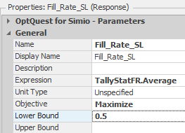
Figure 10.36: Change the Lower Bound on the Service Level
10.8.10 Save and run the model. After the model runs, sort the checked column in descending order to show all the points created on the frontier, as seen in Figure 10.34. Figure 10.38 shows the frontier graphed by copying the data to Excel. The data in Excel has had its duplicates removed and been sorted in descending order.
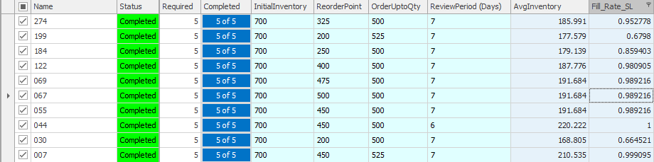
Figure 10.37: Part of the Points Generated on the Pattern Frontier by SIMIO
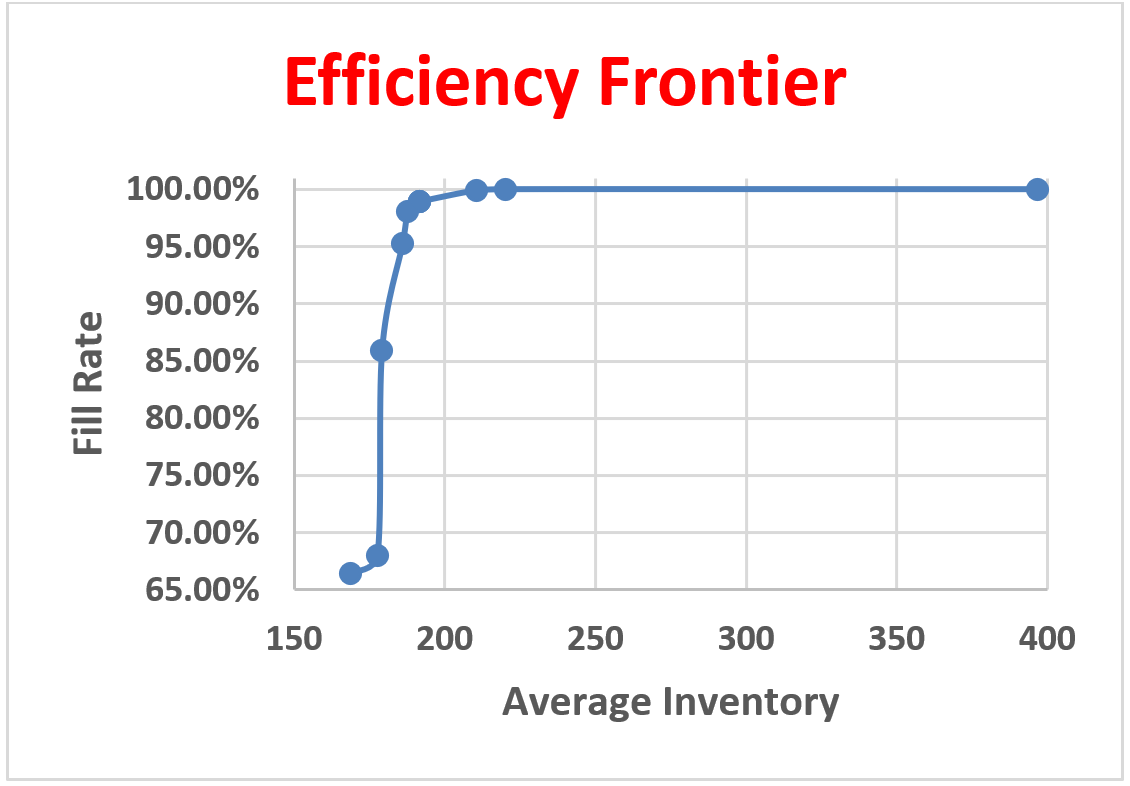
Figure 10.38: Pattern Frontier Graphed in Excel
10.8.11 Note that more complicated constraints can be composed on the inputs (controls). These constraints are more common. A nonsensical example of a constraint on an input in this model could be (ReorderPoint + 3OrderUpToQty >=1000), which is inserted by selecting the Add Constraint* button and entering the equation as seen in Figure 10.39.
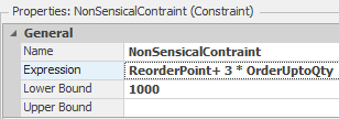
Figure 10.39: Example of Constraint on Decision Variables
10.9 Commentary
- The use of the subset selection facilitates finding a good collection of solutions. The KN ranking and selection scheme is quite good for statistically determining the best scenario for many control variables and scenarios.
- OptQuest is an outstanding optimizer, given enough time and replications. However, the SMORES, subset selection, and KN greatly help determine what “solution” you think is best.
- With the Cost Financials added to SIMIO, one could have optimized cost as well.
Select the ModelEntity in the [Navigation] panel and go the Definitions→States section to add the integer state variable.↩︎
. The first time, you will need to type the category name “Inventory,” which can then be selected from the dropdown box.↩︎
One maybe inclined to use ModelEntity.OrderAmt*Random.Triangular(10,20,30) for the Processing Time property. However, this will not correctly model the summed distribution as seen in the example in Appendix A.↩︎
Inventory position is defined as on-hand inventory plus on-order inventory (to account for orders that haven’t arrived).↩︎
Some may argue this service level calculation is really a fill rate, if the inventory is greater than the order amount then 100% of the demand appears to be satisfied.↩︎
The advantage of using a status table rather than a series of status labels is that you only need to update the table to remove or add metrics to track which could be linked to a spreadsheet.↩︎
The Create step can create new objects or copies of the associated or parent objects. Each of the created objects will be executed by their own token. Note that created tokens are updated in SIMIO before the original.↩︎
When entities are created, they are placed in “FreeSpace” and, typically, will need to be “transferred” from there to one of the model nodes or stations.↩︎
The syntax for the format function is String.Format(string, arg1, arg2, …) where the format “string” can contain place holders that are enclosed by {} which start with the 0th argument (i.e., {0}). For example, String.Format(“SL = {0} and the Avg = {1}", 0.45, 89.4)”)` has two arguments {0} and {1} and replaces those with the numbers 0.45 and 89.4 respectively to produce a ‘SL=0.45 and the Avg = 89.4’. Along with the arguments, one can specify formatting information especially as applied to numbers by using a colon on the argument then specifying the number format. For example, {0:#.##} will display only two significant digits while {0:#.00%} will display a percentage and force there to always be two significant digits.↩︎
Other control variables can be defined.↩︎
The values in the response that don’t fall within the bounds are shown in a red gradient color.↩︎
Refer back to Chapter 8 for more explanation of SMORE plots and their meanings.↩︎
S. Kim and B. L. Nelson, "A Fully Sequential Procedure for Indifference-Zone Selection in Simulation," ACM Transactions on Modeling and Computer Simulation 11 (2001), 251-273.↩︎
Sijia Ma, Shane G. Henderson, “Predicting the Simulation Budget in Ranking and Selection Procedures,” ACM Transactions on Modeling and Computer Simulation 29(3): 14:1-14:25 (2019)↩︎
OptQuest is an additional add-in that has to be purchased.↩︎
Finer resolutions (i.e., smaller values) may lead to better solutions. However, this can affect the solution quality of the optimization algorithm. Having a course resolution quickly allows the algorithm to find a good region. A second optimization with a finer resolution could be run around the point found by the first optimization problem.↩︎
Right click the experiment name in the [Navigation] window to access the properties of the experiment.↩︎
The frontier for two responses is a line and difficult to generate while three would be a plane needing a large number of scenarios.↩︎