Simulation Modeling with Simio - 6th Edition
Chapter
8
Working with Flow and Capacity: The DMV
Almost every object in the SIMIO standard library has capacity, which means that their capacity may be seized and released, typically within the flow of entities - but the Server and the Resource objects are used the most often. As seen in earlier examples, the Server is often the basic flow component of many models. When the Resource has been employed, it is often a secondary resource to a Server. However, their relationship can be convoluted by the need to consider systems with multiple capacities in the context of complicated entity flow.
The Server object is composed of three stations (locations) where entities are held (i.e., InputBuffer, Processing, and OutputBuffer). The stations are animated with “contents” queues, each having its own capacity (see Figure 8.1). A BasicNode is used as input to the Server, while a TransferNode is the output.
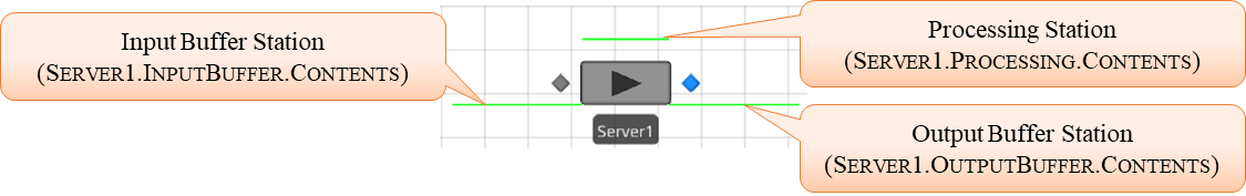
Figure 8.1: The Server Object
The capacity of the Server can be a fixed value or have its capacity controlled by a WorkSchedule. Recall that capacity refers to the number of entities that the object can simultaneously serve. When no capacity of the processing station is available and an InputBuffer exits (i.e., Input Buffer capacity is greater than zero), then the entities wait in the InputBuffer. The Processing Time property is the time required for the server to process an entity in the processing station and is a required property of the server.89 The Server can occupy one of nine states, as explained in Figure 8.2 and SIMIO provides additional symbols to animate the server’s current state automatically. The state applies to all its capacity (i.e., if one or more units of its capacity are allocated, the server is considered processing), and statistics are collected on the amount of time spent in each state.
A Resource is a much simpler object than the Server, but it shares a lot of common properties, including capacity specification, and is not composed of stations. Therefore, a Resource has no place for entities to wait or be served, and no processing time specification is used to control when the resource is released. So, a resource must have its capacity seized and released externally in a SIMIO process, as seen previously.
Flow and capacity are often the primary concerns in many different types of systems (i.e., production, manufacturing, service, healthcare, etc.). Capacity may be used to restrict flow but cannot be arbitrarily expanded. So, finding ways to expand capacity and extend flow is a significant challenge, as simulation offers one way to experiment with different configurations of capacity and different flow mechanisms.
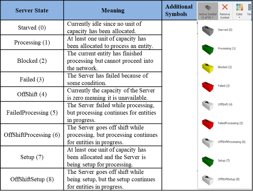
Figure 8.2: Active Symbol Definitions
8.1 The DMV Office
A Department of Motor Vehicles (DMV) often operates multiple offices at various sites across a state. If a simulation model can be created for one site, then perhaps it can be “reused,” with some minor changes, for other sites (and thus, the cost of model development is spread over several installations). A typical DMV office tests driver license applicants and supplies driver licenses to those passing the tests. A typical office size is being used as a reference for the analysis. The office typically opens at 8:30 am and closes at 4:30 pm each day to service license applicants. Applicants arrive more or less randomly, although the rates of arrival change during the day. There are three types of license applicants: Permit, New License, and Renewal. All arriving applicants go through registration, where one of the DMV clerks enters an applicant’s personal information into the computer and collects the license fee. Next, all applicants take a written and visual test on one of three test stations, each of which is staffed by its own DMV Tester. Not everyone passes these tests. Those getting a “New License” must also pass a driving test accompanied by a DMV officer, where some fail the driving test. People who fail any (written/visual or driving) of the tests leave the office and return another day. Those who pass all their tests have their picture taken and their license processed and printed. The DMV is interested in the office's service to applicants and the use of DMV resources. Consequently, the flow times of applicants are a major concern. Since queuing times are a part of flow time, it is important. If congestion in the office becomes high, this also becomes a concern. Finally, since these are public facilities, the cost of the facilities, especially the use of DMV resources, must be balanced against the service to applicants.
Developing a Base Model
In any modeling activity, try to start with the simplest model you can develop quickly. Make whatever assumptions you need to get a model “up and running” right away. It’s alright if your assumptions don’t correspond to reality. We want something to work because we want to extend and evolve our model rather than create a final model at the beginning. Most people new to simulation modeling want their model to be close to the final one, even though it is their initial attempt. They discover that their model has all kinds of complexities that they have trouble unraveling when they encounter an error. Suppose they started with a simple (maybe completely unrealistic) model that is working. In that case, they can embellish it incrementally and adapt it into a final working model with far less difficulty than trying to create the final model at the beginning. Finally, it is not possible to build a model that ultimately represents the real system in every detail. If that is your plan, then you are better off experimenting with the real system. Remember, a model is only an approximation of the real system. How detailed your model is depends on what you want the model to reveal. In general, your model needs only to be as detailed as needed to obtain the performance measures of interest. Any more detail is unnecessary.90
A second recommendation is not to worry about the input right away. The critical concern is getting a model that appears most closely to match the system so you can reliably obtain the needed performance measures. As you are building your model, it will become clear what input data is needed. Let the model inform your data collection so you don’t spend a lot of time collecting unimportant or wrong data.
8.1.1 Draw a flowchart of the service process, which can come from a “value-stream map”.
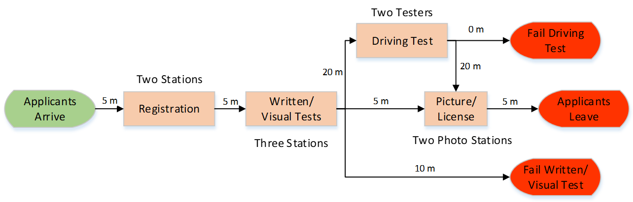
Figure 8.3: DMV Flowchart
8.1.2 Since our flowchart in Figure 8.3 corresponds easily to the basic SIMIO objects, it can be used as a basis for the initial model. Use the following information to create a model with the appropriate objects as shown in Figure 8.4.
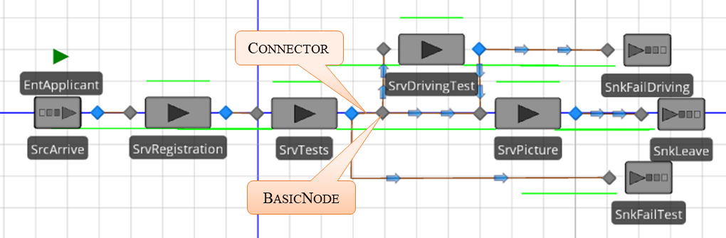
Figure 8.4: Initial DMV Model
- Insert a new ModelEntity named EntApplicants with the Initial Desired Speed property set to “1” meter per second. The applicants arrive randomly but in a time-varying arrival process. Based on this information, general estimates of the arrival rates are shown in Table 8.1. From the Data tab, insert a new Rate Table named ArrivalRateTable that has 15 intervals with an interval size of 30 minutes.
| Time | Hourly Arrival Rate |
|---|---|
| 8:30 – 9 am | 15 |
| 9 – 9:30 am | 10 |
| 9:30 – 10 am | 8 |
| 10 – 10:30 am | 12 |
| 10:30 – 11 am | 15 |
| 11:00 – 11:30 am | 18 |
| 11:30 – noon | 15 |
| Noon – 12:30 pm | 12 |
| 12:30 – 1 pm | 10 |
| 1 – 1:30 pm | 8 |
| 1:30 – 2 pm | 6 |
| 2 – 2:30 pm | 7 |
| 2:30 – 3 pm | 5 |
| 3:00 – 3:30 pm | 5 |
| 3:30 – 4 pm | 5 |
- Insert a new Source named SrcArrive that uses the new arrival table ArrivalRateTable.
- The four basic activities will be modeled using Servers named SrvRegistration, SrvTests, SrvDrivingTest, and SrvPicture, as seen in Figure 8.4.
- From Figure 8.4, notice the BasicNode named BNodePass that was inserted after SrvTests, which is not part of the flow chart but will be used to help branch applicants who fail the written or eye test. Use a Connector between the SrcTests Server and the BasicNode so it doesn’t take any time. Use a 20-meter and a five-meter path between the BasicNode and SrvDrivingTest and SrvPicture, respectively. Connect all other objects via paths based on the distances from the flow chart.
- Finally, insert three Sinks named SnkLeave, SnkFailTest, and SnkFailDriving.91
8.1.3 Recall there are three types of applicants (i.e., permits, new licenses, and renewal licenses).
- To keep track of time in the system for each type, insert a Tally Statistic, as seen in Figure 8.5. Make sure your Tally statistics have Time as the Unit Type.
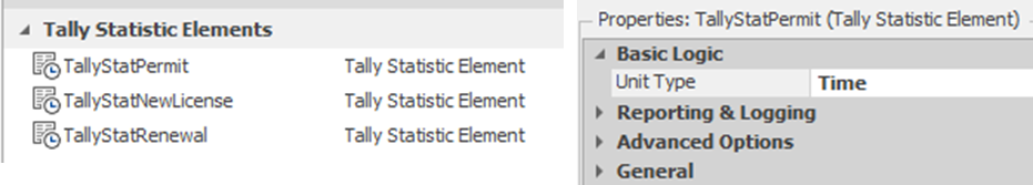
Figure 8.5: Creating Tally Statistics to Track Time in the System for Each Type of Applicant
- Insert a new data table from the Data tab named TableApplicant with six different properties with the following particular characteristics defined in Table 8.2 and shown in Figure 8.6.
| Property Name | Property Type | Description |
|---|---|---|
| Name | String | The name of the applicant type |
| ApplicantType | Integer | It will be used to set the entity’s animation picture |
| ApplicantMix | Real | The percentage of time this applicant type arrives |
| RegistrationTime | Expression (Unit Type set to “Time” with minutes as the Default Units). | The registration time varies by the applicant type. |
| PassTests | Real | The probability of passing varies by applicant type |
| PassDrivingTest | Real | Probability of passing the driving test |
| TallyStatTimeInSystem | Tally Statistics Element | Used to track each type’s time in system |
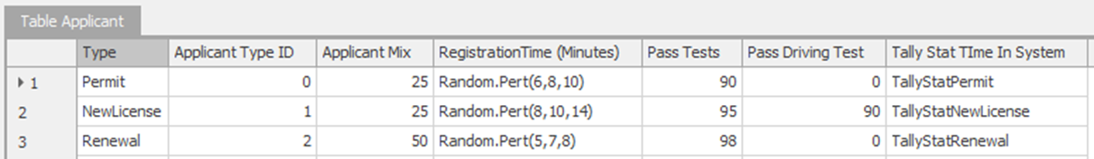
Figure 8.6: Table Values for the Three Applicant Types
- Select the EntApplicant and add two additional symbols, coloring them red and blue, respectively.92
- Next, as EntApplicants are created by the SrcArrive, assign the applicant type and associated picture using the Created Entity Add-on Process Trigger, as seen in Figure 8.7.93
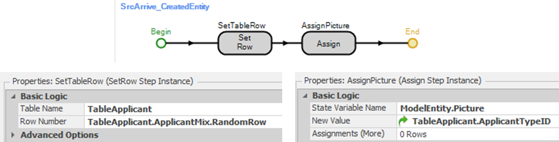
Figure 8.7: Assigning the Applicant Type and Picture
- Once applicants leave the system, tally the time in the system through the Entered Add-on Process Trigger of the SnkLeave, as shown in Figure 8.8.
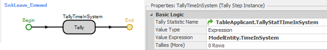
Figure 8.8: Tally Time in System
8.1.4 Use Table 8.3 to set the processing times and capacities for each of the four servers.
| Server | Processing Time Property Value | Initial Capacity |
|---|---|---|
| SrvRegistration | TableApplicant.RegistationTime | 2 |
| SrvTests | Pert(10, 14, 20) minutes | 3 |
| SrvDrivingTest | Pert(15, 25, 40) minutes | 2 |
| SrvPicture | Pert(1, 2, 3) minutes | 2 |
8.1.5 If you save and run the model, the applicants will choose the various branches equally likely since the Selection Weight properties are all set to one. Recall that only new licenses go through the driving test, and the passing rate of the driving and written/eye tests are stored in the table. Change the Selection Weight properties for the paths so they account for how the applicant types should branch, as seen in Table 8.4.
| From Node | To Node | Selection Weight Property |
|---|---|---|
| Output@SrvTests | BasicNode named BNodePass | TableApplicant.PassTests |
| Output@SrvTests | Input@SnkFailTests | 100 – TableApplicant.PassTests |
| BNodePass | Input@SrvDrivingTest | TableApplicant.ApplicantTypeID == 1 |
| BNodePass | Input@SrvPicture | TableApplicant.ApplicantTypeID != 1 |
| Output@SrvDrivingTest | Input@SrvPicture | TableApplicant.PassDrivingTest |
| Output@SrvDrivingTest | Input@SnkFailDriving | 100 – TableApplicant.PassDrivingTest |
8.1.6 Save and run the model, observing it for a while before fast-forwarding to complete one replication.
8.1.6.1 What are the average times in system for New License, Permit, and Renewal applicants?
_______________________________________________
8.1.6.2 What are the stations' observed “ScheduledUtilization” for Driving Tests, taking Pictures, Registration, and Tests?
_______________________________________________
8.1.6.3 Do you have any concerns relative to the model's behavior or the results?
_______________________________________________
8.2 Using Resources with Servers
After building the initial model, it was discovered that the people who register applicants also take pictures and hand out the licenses. These DMV clerks work in the same physical area and share the workload, meaning there are four clerks to perform both functions. However, when we ask about the working environment, we find that only three applicants can be processed at once at the registration and that only two people can have their picture taken at the same time.
8.2.1 Change the capacity of the SrvRegistration to three, meaning that no more than three entities can be processed at the same time on this server. The SrvPicture’s capacity will remain two.
8.2.2 Insert a Resource object into the model named ResClerks with an initial capacity of four, which corresponds to the four clerks. A resource object can have its capacity “used” at several servers within a model, while server capacity is limited to a specific server.
8.2.3 Next, under the Secondary Resources94 section at both the SrvRegistration and SrvPicture servers, use the “Resource for Processing” property and specify the use of ResClerks95, as seen in Figure 8.9.
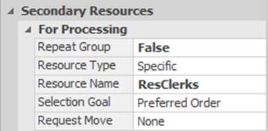
Figure 8.9: Specifying the use of Clerks at the Server
8.2.4 Save and run the model.
8.2.4.2 Did you notice that the Resource shows its “Busy (1)” state whenever any of its capacity is being used, similar to the Processing state of the server?
_______________________________________________
If a server employs resources for service, then the capacity to serve entities may be limited by either the resource capacity availability, the server capacity availability, or both. If only resources limit the capacity, then the server capacity should be made arbitrarily large (i.e., infinity) so as to not constrain the system.
8.3 Handling Failures
Suppose we now discover that the reception area is interrupted by phone calls. These phone calls arrive randomly (i.e., Exponentially distributed) on average every 30 minutes, and they take anywhere from 1 to 4 minutes, with 2 minutes being typical.
Both Servers and Resources can experience failures, as can Workstations, Combiners, Separators, Vehicles, and Workers. The failure options are found under the object’s “Reliability Logic” property section. In SIMIO, the failure concept is intended to be used for any downtime, exception, or (non-modeled) interruption96. Four different types of failures can be specified, two of which are based on “counts” while the others are based on time, as described in Table 8.5.
| Failure Type | Description |
|---|---|
| No Failures | No failure or exception will occur. |
| Calendar Time Based | The user specifies the time between exceptions or failures. Often used model general reliability or maintenance programs. |
| Event Count Based | The user specifies that an exception or failure will occur after a particular number of events has happened (e.g., the number of tool changes or a specific number of arrivals). |
| Processing Count Based | The user specifies that an exception or failure will occur after a certain number of operations have occurred on the Server. |
| Processing Time Based | The user specifies that an exception or failure will occur after the object has operated a certain amount of time (e.g., after 100 hours of operation the machine has to go through maintenance). |
When an object is interrupted, its entire capacity is interrupted – its state is changed to “Failed(3)”. So, do we interrupt the service at the server, or do we interrupt the resource?
8.3.1 One can use a “Calendar Time Based” type failure to model the phone call interruption. Select the SrvRegistration Server object and specify the “reliability logic,” as shown in Figure 8.10, using the Uptime Between Failure and the Time to Repair expressions corresponding to the phone calls.
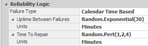
Figure 8.10: Specifying the Failure
8.3.2 Implement this reliability logic in the SrvRegistration. Run the model and observe its behavior.
8.3.2.1 Did you see the interruptions displayed by the server being colored red?
_______________________________________________
8.3.2.2 If you simulate in fast-forward, the simulation ends at 7.5 hours; how many phone calls were handled at the registration desk, and what percent of the time did the registration desk fail?
_______________________________________________
8.3.3 In reality, the clerks are the ones that need to answer the phone calls. Take the failure off the server and put it on the resource ResClerks. Run the model and observe its behavior.
8.3.4 If you simulate in fast-forward, the simulation ends in 7.5 hours. Examine the resource statistics for ResClerks, and you will notice “TimeFailed” and “TimeFailedBusy” state statistics. The “Failed(3)” state occurs when the resource is not busy, and the “FailedBusy(5)” state occurs when it is busy (at least one unit of capacity is being used). Notice that the colors for both states are the same, so you can’t tell between the two failed states in the animation.
8.3.4.1 From the statistics on the resource, how many phone calls were handled by the resource when it was idle, and how many phone calls were handled when the resource was busy?
_______________________________________________
8.3.5 Unfortunately, failing the entire server or resource is probably not our best option for modeling the handling of phone calls. Since the phone calls are answered individually, we need to spread them over the clerks. One possibility would be to create entities to represent the phone calls and have them interrupt existing service. However, let’s use the pre-defined reliability logic for our present purposes. However, each clerk needs to handle phone calls individually, so we need to have individual resources. Replace our ResClerks with four separate Resource objects, each with capacity one (see Figure 8.11). Since phone calls occur about 30 minutes apart (on average), we will specify the time between phone calls to be 120 minutes for each clerk, using the previous time to repair.97
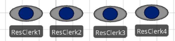
Figure 8.11: Individual Clerks
8.3.6 Unfortunately, secondary resources98 can only seize a single specific object (i.e., the ResClerks, which had a capacity of four), but now there are four separate Resources that need to be seized. From the “Definitions” tab, create an Object List called ListClerks that contains the four clerk Resources, as seen in Figure 8.12. The list will allow us to select one of the clerks based on some criteria.
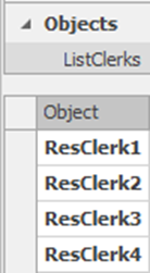
Figure 8.12: Creating an Object List of Resources
8.3.7 At both the SrvRegistration and SrvPicture servers, under the Secondary Resources section for Resource for Processing, choose the “Select From List” option as the Object Type property. Specify the ListClerks as the Object List Name property value, as seen in Figure 8.13. Use “Random” as the Selection Goal, which forces SIMIO to use the clerks at the servers uniformly.
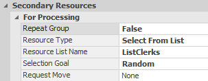
Figure 8.13: Select a Clerk
8.3.8 Save and run the model, look at the animation, and finally, look at the statistics at the end of 7.5 hours. Now, four resources are being modeled, so there are individual statistics for each.
8.3.8.1 What is the scheduled utilization for each of the clerks?
_______________________________________________
8.4 Server Configuration Alternatives
Sometimes, there are desirable alternative configurations for the servers in a model, often motivated by animation needs or handling separate failures. For example, the SrvTests object in the current model represents the processing of up to three applicants at the testing stations. Perhaps it would be better to represent this service as three separate Servers. Also, the evaluators that administer the test need to take a break after processing between eight or twelve applicants, so separate Servers will be needed.
8.4.1 The evaluators that assess the written and eye tests take a break after processing between eight and twelve applicants. The reliability logic can be used to handle this type of break. Set the Failure Type property to “Processing Count Based” to count the number of applicants where the Count Between Failures set to a uniform distribution between eight and twelve with the time of the break taking between two and six minutes, but generally they take four minutes as seen in Figure 8.14.
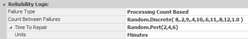
Figure 8.14: Taking a Break Based on the Number of Applicants Processed
8.4.2 Since the evaluators doing the test will not break at the same time, we need to have individual test stations. Change the name of SrvTests to SrvTests2 and the capacity back to “1.” Copy it two times, creating a total of three Server objects, as shown in Figure 8.15. Connect the test stations with the registration using five-meter Paths. We will assume that the branching to each testing station is equally likely (i.e., equal Selection Weights). Connect the other two tests with Connectors to the Ouput@SrvTests2, which allows us to use the same branching logic to drive test, picture taking, or failure.
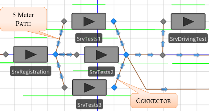
Figure 8.15: Separate Testing Stations
8.4.3 Now save and run this model while observing the animation.
8.4.4 Typically, there is one waiting station after registration where they wait for the next available testing station. To prevent applicants from waiting at the testing stations, first set the input buffer capacity of each testing server to zero under the Buffer Capacities section of the Server object.
8.4.5 Save and rerun the model, observing the animation.
8.4.5.1 Now, how do the applicants wait at the testing stations? Is that a desired behavior?
_______________________________________________
The applicants now wait at the input node of the testing stations and are unable to enter the Server’s station since the input buffer capacity is zero. Furthermore, the entities seem to make a decision about which path to take independent of the traffic on that path, the number at the associated test station, or if the tester is on break.
8.4.6 To handle those issues, the branching process needs to be modified to choose an appropriate testing station. From the “Definitions” tab, create a Node List called ListTesters that contains the input node (i.e., Input@) for each of the three testers, as seen in Figure 8.16. A list will allow SIMIO to select one of the input nodes using some criterion.
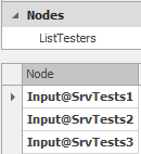
Figure 8.16: Creating a Node List of Testers
8.4.7 Select the Output@SrvRegistration transfer node that connects the registration to the servers, change the Entity Destination Type property to “Select From List,” and select the ListTesters list that was just created in the Node List Name property.
- Set the Selection Goal property to be the Smallest Value with the Selection Expression99 equal to Candidate.Node.AssociatedStationLoad100, which chooses the server with the shortest line by determining the number that is routed to the server plus the number in the Contents Queues of the InputBuffer101 and Processing102 stations, as seen in Figure 8.17.
- If a tester is taking a break, applicants should not be routed to this person while they are on the break. To avoid selecting these nodes, the Select Condition property can be used to include only certain items from a list. This expression property has to evaluate to “True” before the Candidate Node object will be considered for selection for routing. Therefore, we will set the property to select only those servers that have not failed before choosing the smallest line.
- The Failure.Active function will be “False” if the server is currently not in a failure mode. If the server has not failed, then allow it to be selected as a candidate using the expression !Candidate.Server.Failure.Active, as seen in Figure 8.17.103
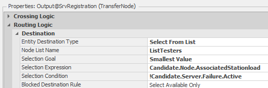
Figure 8.17: Choosing the Shortest Line
8.5 Restricting Entity to Flow to Parallel Servers
Now, applicants are forced to wait in the registration output node until a tester is available (i.e., the Server is empty) because the traveler capacity paths are one, and the server’s input buffers are zero. Chapter 14 will present a more complete explanation of various blocking methods. Sometimes, it is necessary to block flow under somewhat complex circumstances. Suppose that the testers who give the visual and written exam must enter the exam results into a computer. The applicant is allowed to return to the waiting area, but the tester remains busy to complete the process. Obviously, the tester is unavailable to other applicants until the results are entered.
8.5.1 To keep track of the status of the tester, we will utilize a State Variable associated with each tester. From the Definitions→States section, insert a new discrete String state variable named GStaTesterStatus. Since there are three rooms, make the Dimension Type property a Vector and set the number of Rows to three with an Initial State Value of Available104 as seen in Figure 8.18.105
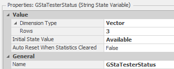
Figure 8.18: Setting a Vector State Variable
8.5.2 From the Animation tab, insert three status labels beside each of the tester Servers with an expression associated with the GStaTesterStatus (e.g., GStaTesterStatus[1] for the first room as seen in Figure 8.19). Specify all three expressions accordingly. Vectors start with an index of one, and each row is specified in brackets.
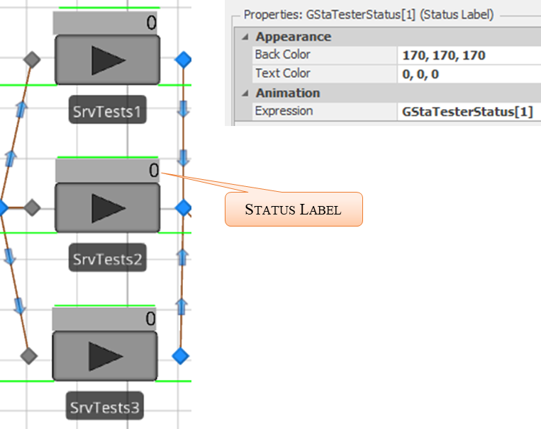
Figure 8.19: Adding Status Labels
8.5.3 Once an applicant has been seen by one of the testers, we will need to set the status of the tester to “DataEntry,” delay for five to ten minutes, and then set the status to “Available.” We will model this via a specialized process for each room. Navigate to the “Processes” Tab from the Process section, and use the Create Process button to create a new process named ProcessDataEntry, as seen in Figure 8.20. Note that this is a case where State Assignments cannot be used to model the scenario.
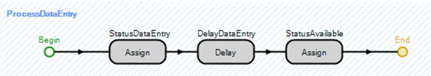
Figure 8.20: Process for Data Entry and Changing the Status of the Tester
- Insert an Assign step that will set the first room’s status (i.e., GStaTesterStatus[1] to “DataEntry”.
- Insert a Delay step with a Delay Time expression set to Random.Uniform(3,6). For a moment, we will leave the Units set to hours, which allows us to see any potential problems.
- Copy the first Assign step and change the Value to “Available.”
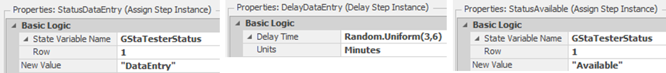
Figure 8.21: Process Steps and Values for ProcessDataEntry
8.5.4 The new process needs to be invoked after the applicant has finished processing. In the Facility window, select SrvTests1 and specify the ProcessDataEntry1 as the After Processing add-on process trigger which is invoked immediately after the entity has finished processing.
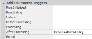
Figure 8.22: Using the ProcessDataEntry as the After Processing Add-On Process Trigger
8.5.6 You should have noticed that the entity does not leave the tester until after the data entry is complete, which is not what we wanted. The reason this occurs is that the ModelEntity is delayed, and not just the tester. The Exited add-on process trigger is invoked after the entity has physically left the Server. Instead of using the After Processing, specify the ProcessDataEntry process as the Exited add-on process trigger.
8.5.8 What happens to the next applicant waiting for this tester?
_______________________________________________
In the first case, the current entity was delayed and did not leave the tester. When using the Exited trigger, the current applicant leaves the room, but the next applicant is not blocked, will enter the tester and begin processing. Also, the tester's utilization is incorrect because they are idle when performing the data entry.
8.5.9 Therefore, we need to seize the tester to prevent it from being freed when the applicant leaves the room and release the server once the data entry is finished. Insert a Seize and Release steps to the ProcessDataEntry process as shown in Figure 8.23.

Figure 8.23: Adding a Seize and Release of Tester1
- Because the entity has left the server, it cannot be used to seize the tester. Therefore, we will use the ParentObject, which is the Model in this scenario, as the Owner Type, for both the Seize and Release process steps, as seen in Figure 8.24.
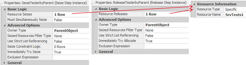
Figure 8.24: Seize and Release SrvTest1 by ParentObject
8.5.11 The entities are still allowed to enter the path to the server even though the server is busy. Therefore, we need to block the server or the path using a different mechanism.106 We need to edit the Routing Logic for the Output@Registration TransferNode. Recall the Selection Condition property of the Routing Logic section, which must evaluate as “True” in order for that particular node to be selected. Currently, the condition will not select testers that have failed. Therefore, modify the condition to include not choosing servers that are currently processing (i.e., resource state equal to one), as seen in Figure 8.25.
!Candidate.Server.Failure.Active && Candidate.Server.ResourceState!=1107
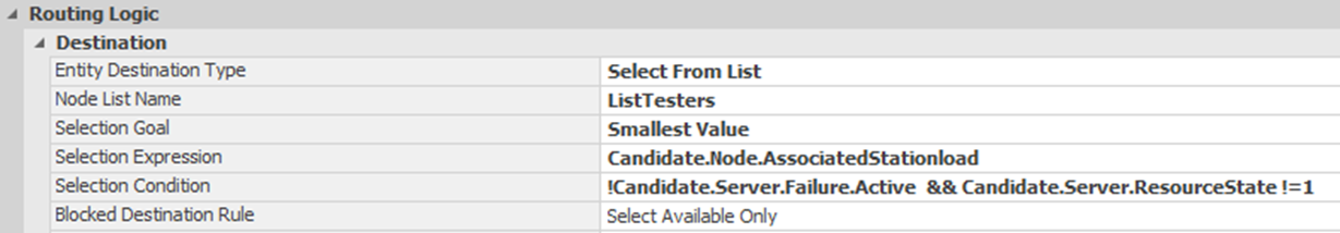
Figure 8.25: TransferNode: Setting Traveler Capacity
8.5.12 Save and run to make sure that the Server does not accept entities now.
8.5.13 Since the model is working properly now, change the Units of time to “Minutes” for the Delay step of ProcessDataEntry.
8.5.14 At this point, we could select the ProcessDataEntry process and copy it two times. Then change the names of the two copied processes to ProcessDataEntry2 and ProcessDataEntry3, the two Assign steps (i.e., the Row property set to two or three), the Seize step, and the Release step to specify the correct tester. However, to do this more generally (i.e., have the same process used by all three testers), we will use a “Tokenized Process.” This approach will be especially useful if additional testing stations are added later.
- From the Definitions tab, define a new Token named TknTester. Add an Integer state variable named TStaWhichRowNumber, and from the Object Reference section, add an Object Reference state variable named TStaWhichTester, as seen in Figure 8.26.
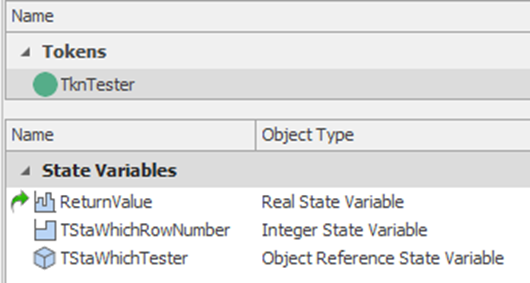
Figure 8.26: New Token TnkTester to be used in a Tokenized Process
- Edit the ProcessDataEntry process. Modify the process’s Advanced Options properties by specifying the process that will be executed by the TknTester token, as shown in Figure 8.27. Next, specify the process will take two input arguments (i.e., WhichRowNumber linked to TknTester.TStaWhichRowNumber and WhichTester linked to TnkTexter.TStaWhichTester).
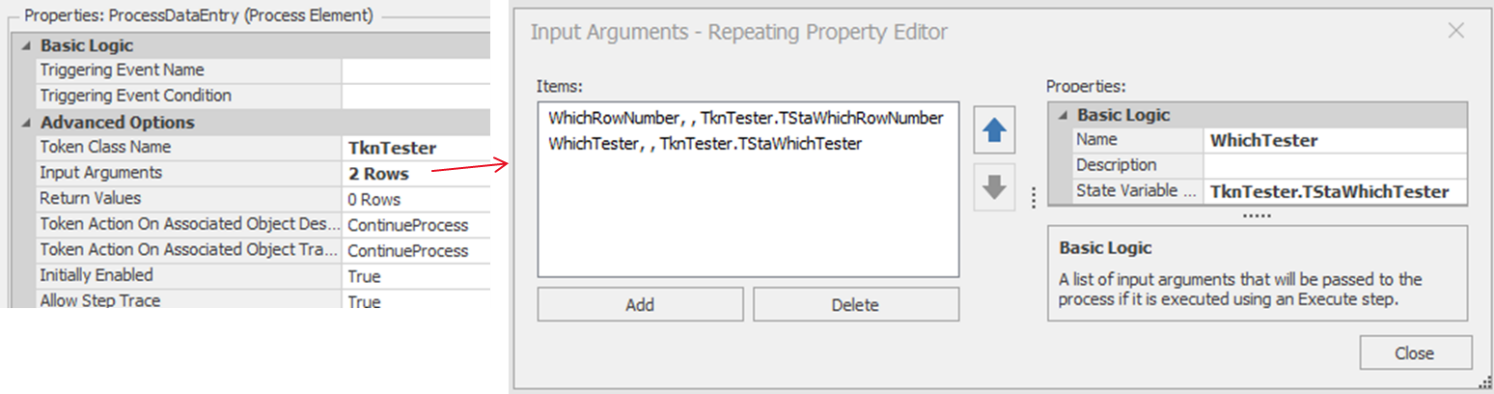
Figure 8.27: Adding Token Information to the Process
8.5.15 Next, change the two Assign steps within the process to employ the TStaWhichRowNumber as the Row property to update the GStaTesterStatus passed to the token TknTester, as seen in Figure 8.28.
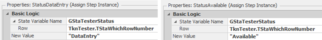
Figure 8.28: Use the Token Argument
8.5.16 Update the Seize and Release steps to use TStaWhichTester as the specific Object Name.
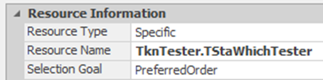
Figure 8.29: Using the TknTester to Specify Which Server to Seize and Release
8.5.17 From the facility window, select SrvTests1 and set the Exited add-on process trigger, as seen in Figure 8.33, to pass in the correct row number and tester. Repeat this for the other two testers, setting the row number and which tester to the correct values (i.e., “2” and “3” and SrvTests2 and SrvTests3, respectively).
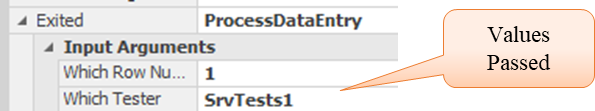
Figure 8.30: Invoking the Exited Process with its Argument
8.5.18 The status labels currently change from “Available” to “Data Entry” but remain “Available” while the Server is processing an applicant. We need to update the status to busy when the tester is servicing an applicant to fix this issue.
- Since it will be similar for all three testers, add another “Tokenized Process” named ChangeStatustoBusy, as seen in Figure 8.31. Next, use the Token TknTester as the Token Class Name property and insert one input argument (i.e., the row number).
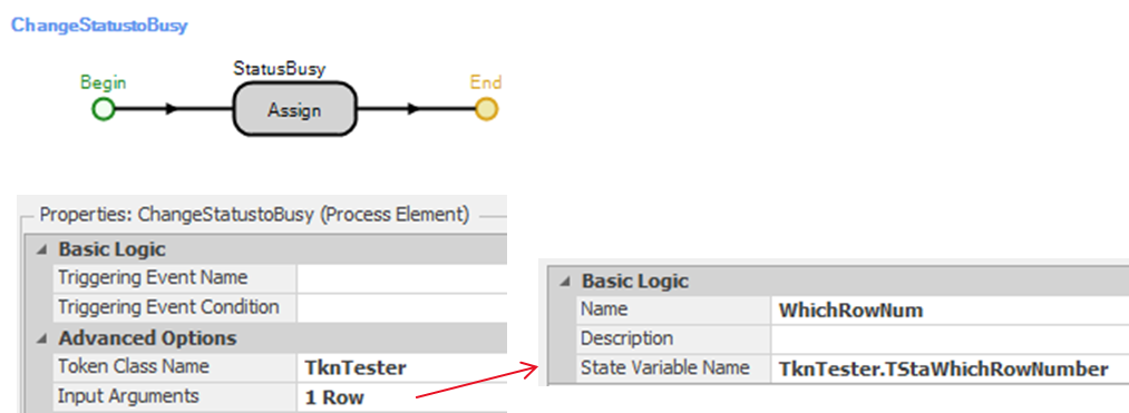
Figure 8.31: Creating the Process that will update the Status to Busy
- Insert an Assign step that will set the GStaTesterStatus variable to “Busy,” as seen in Figure 8.32.

Figure 8.32: Setting the Status to Busy in the Assign Step
8.5.19 For each of the three tester Servers, specify the Before Processing Add-on Process triggers to use the ChangeStatustoBusy process specifying the correct row number, as seen in Figure 8.33 for the first tester.
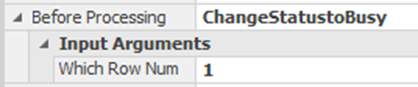
Figure 8.33: Changing the Room Status to Busy
8.5.20 Save and run the model, ensuring the status labels turn to “Busy,” and the model works correctly.
8.5.20.1 What is the average utilization of each server?
_______________________________________________
8.5.20.2 What is the total time an applicant has to wait for a tester?
_______________________________________________
8.6 The Waiting Room Size
In the real system, people wait for services in a common waiting area, except for those waiting for registration, who queue in front of the registration. This common area consists of waiting for the tester, the driving test, and the picture/license. Looking at each waiting area separately ignores the fact that contributions to the waiting area change throughout the day. To visually see what is happening in the common waiting area, we need to introduce the SIMIO Storage object, which will be used to represent all the waiting areas together. (Storages do not actually contain entities, but entities hold membership in storages.)
8.6.1 From the Definitions→Elements section, insert a new “General” Storage element named StoWaitingRoom.
8.6.2 Entries (i.e., entities) are added to Storage elements via an Insert step and removed via the Remove step. Add two new processes named WaitingRoomEntered and WaitingRoomExited, as seen in Figure 8.34 and Figure 8.35, respectively. Specify the StoWaitingRoom.Queue as the Queue State Name property.

Figure 8.34: Inserting into the WaitingRoom
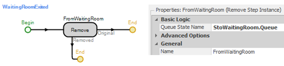
Figure 8.35: Removing from the WaitingRoom
8.6.3 People enter the common waiting room when they leave the registration desk or when they are waiting at the driving test or the picture area.
- For the After Processing add-on process trigger of the SrvRegistration, specify the WaitingRoomEntered process.
- Select both the SrvDrivingTest and SrvPicture and then specify the WaitingRoomEntered process as the Entered add-on process trigger.
8.6.4 People leave the waiting room when they enter service at the testers, driving test, or picture area.
- Select both the SrvDrivingTest and SrvPicture, then specify the WaitingRoomExited process as the Before Processing add-on process trigger.
- For the three testers (i.e., SrvTests1, SrvTests2, and SrvTests3), we will need to modify the ChangeStatustoBusy process since it is already specified as the Before Processing add-on process trigger. Insert an Execute step with the Process Name specified as WaitingRoomExited.
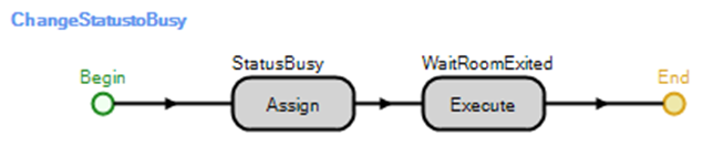
Figure 8.36: Using Execute Step to Cause Applicants to Leave the Common Area
8.6.5 To “see” the waiting room, insert a DetachedQueue from the Animation tab. The Queue State property for the queue is the StoWaitingRoom.Queue. Draw a straight line for the queue.
8.6.6 Most waiting rooms have people along the edge of a room rather than a straight line.108
- Select the animated WaitingRoom queue, which is the green straight line by default.
- Change the Alignment to Oriented Point and then select the Keep in Place option since entities, once they sit, will not keep changing seats along the queue like a checkout line does, as seen in Figure 8.37.
- From the Vertices section, add two vertices by selecting the Add Vertex button and dragging the green vertex onto the queue.
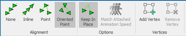
Figure 8.37: Adding an Animated Queue
- Form a U-shaped queue by moving the two new vertex points that were just added to the appropriate spots. Then continue adding vertexes and then moving the points inward to form the waiting room queue as seen in Figure 8.38.
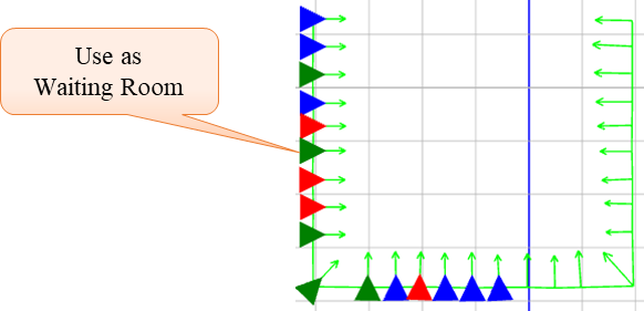
Figure 8.38: Adding an Animated Queue in a Different Shape
8.7 Using Appointment Schedules
In response to applicant waiting concerns, the office has decided to offer a few scheduled appointments to provide better service to the applicants. The office will still allow most people to “walk-in” but will prioritize those with an appointment. In particular, the office will schedule applicants for the following nine appointment times during the day: 8:30 am, 9:00 am, 9:30 am, 10:00 am, 2:00 pm, 2:30 pm, 3:00 pm, and 3:30 pm. The appointments are scheduled for applicants when there are lower arrival rates. Some applicants who have appointments will arrive early, while others may arrive late, which is called “early/late” arrivals. Also, it is expected that some may skip their appointment altogether (i.e., “no-shows”).
You need to realize that a “scheduled arrival process” is fundamentally different from the usual “random” arrival process in that the random arrival process has random interarrival times while the scheduled arrival process has known interarrival times. Randomness in the scheduled arrival process occurs in the early/late arrivals and the no-shows. In many “service industries,” scheduled arrival processes are more prevalent than random arrivals.
8.7.1 The scheduled appointment times are specified via a data table. From the Data tab, add a new data table named TableArrivals. Insert a Date Time column named ScheduledTime from the Standard Property drop-down, as seen in Figure 8.39. Next, specify the scheduled appointments, which indicate the time of arrival.109 At this point, these appointments are absolute arrival times (i.e., if the simulation was to start on 9/5/2015 instead of 9/6/2015, no arrivals would occur until the next day, or if the simulation start date was 9/7/2015, then no arrivals would occur). See the Commentary section at the end of the chapter on specifying a table with relative time offsets.
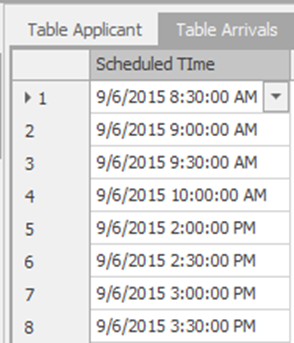
Figure 8.39: Specifying the Appointments
8.7.2 Since we assume one person will arrive at the scheduled appointments, we will reduce the arrival rate table by one for the first and last four time periods so comparisons can be made, as shown in the Table 8.6 .
| Time | Hourly Arrival Rate |
|---|---|
| 8:30-9 am | 14 |
| 9-9:30 am | 9 |
| 9:30-10 am | 7 |
| 10-10:30 am | 11 |
| Middle Times Unaffected | |
| 2-2:30 pm | 6 |
| 2:30-3 pm | 4 |
| 3:00-3:30 pm | 4 |
| 3:30-4 pm | 4 |
8.7.3 In the Facility tab, insert a new Source object named SrcScheduledArrivals, as shown in Figure 8.40. Next, it is connected to the output node of the original Source via a Connector, which allows arrivals to originate from one point and travel along the same five meter path to the reception area.
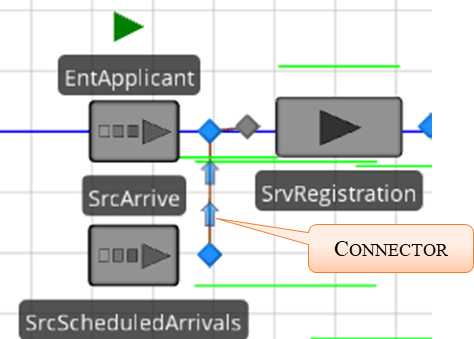
Figure 8.40: Adding an Additional Source to Handle the Scheduled Appointments
8.7.4 To utilize appointment schedules, change the Arrival Mode to “Arrival Table” and specify the Arrival Time Property as the column TableArrivals.ScheduledTime as seen in Figure 8.41.
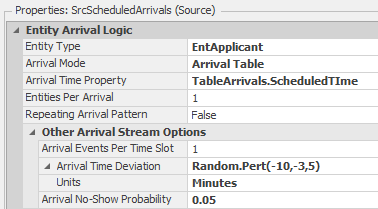
Figure 8.41: Specifying the Appointment Scheduling in the Source
8.7.5 The Arrival Time Deviation property is used to model the deviation from the appointed scheduled time specified by the TableArrivals.ScheduledTime. In this example, we are stating that applicants can arrive as early as ten minutes or as late as five minutes, but most will arrive three minutes early, using a Pert distribution110. See Table 8.7 for an explanation of all the appointment schedule properties.
| Appointment Scheduled Property | Description |
|---|---|
| Arrival Time Property | The numeric table property specifies the list of scheduled arrival times, which can be a Date Time or any numeric or expression property. |
| Arrival Events Per Time Slot | This is the expected number of arrival events that will occur at each arrival time. You can think of this as how many batches will arrive, where the Entities Per Arrival will determine the number of Entities per batch that will arrive. |
| Arrival Time Deviation | It specifies the deviation from the scheduled time, which affects each batch differently. Therefore, two Arrival Events Per Time Slot and 1 Entities Per Arrival will be different than one Arrival Event Per Time Slot and 2 Entities Per Arrival. When a deviation or no-show probability is specified, as in the latter case, the two entities will always arrive at the same time. |
| Arrival No-Show Probability | Specify the probability of a no-show occurring, which is applied to a batch arrival. |
| Entities Per Arrival | The number of entities to create for each batch. |
| Repeat Arrival Pattern | When you reach the end of the table, determine whether or not to repeat the pattern. If you have specified actual times, these are converted to deviations or time offsets. For this example, the first arrival is at 12 pm, with the simulation starting at 11 am, which means there is a 1 hour time offset till the first arrival. So, at 4 pm, when the last scheduled arrival occurs, the simulation will start back up with arrivals at 5 pm to have the same offset if this property is set to “True.” |
8.7.6 In this case, we assume 5% of the applicants are “no-shows” and skip their appointments. Therefore, set the Arrival No-Show Probability property to 0.05.
8.7.7 In the SrcScheduledArrivals source reference, the process SrcArrive_CreatedEntity is used as the Created Entity add-on process trigger. Also, in order to distinguish the scheduled arrivals, assign the ModelEntity.Priority a value “2” in the Before Exiting of the “State Assignments” section. Recall the default Priority state variable has a value of 1.111 Refer to Figure 8.42.
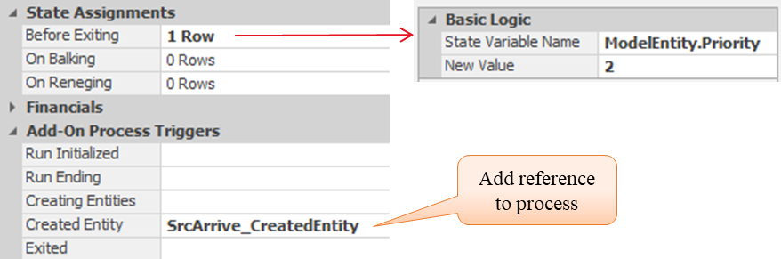
Figure 8.42: Specifying Properties of the SrcScheduledArrivals Source
8.7.8 We would like to keep track of time in the system according to whether the applicant had a scheduled appointment or they were a walk-in. From the Definitions→Elements section, add two Tally Statistics named TallyStatSchedTimeInSystem and TallyStatWalkInTimeInSystem with the Unit Type property set to “Time.”
8.7.9 To obtain the time in system statistics for the two types of arrivals, each needs to be tallied. One way to obtain the tallies is to use the Tally Statistics section of the Input@SnkLeave specifying On Exited, as shown in Figure 8.43.
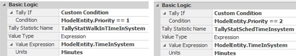
Figure 8.43: Collecting Time in System by Arrival Type
8.7.10 Select the experiment and add a new response for each of the Tally Statistics named WalkInTimeInSystem with an Expression set to
TallyStatWalkInTimeInSystem.Average and ScheduledTimeInSystem with TallyStatSchedTimeInSystem.Average. Both should have a Unit Type as Time with Display Units as Minutes.
8.7.11 Save the current model. Reset the experiment and run for 100 replications.
8.7.12 One of the potential issues is that scheduled patients are not processed differently in the model. Applicants who have scheduled appointments should have a higher priority than walk-in applicants.
- Therefore, select SrvRegistration, SrvDrivingTest, and SrvPicture Servers in the model and change their Ranking Rule property so that scheduled appointments have a larger priority, as seen in Figure 8.44.
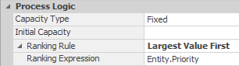
Figure 8.44: Changing the Ranking Rule in the Servers
- For the testing Servers, the expression has to be a little more complicated because both entities and the Model seize server capacity. We need to give priority to the Model for the data entry process using the following expression seen in Figure 8.45. The Is.Entity function will return true if an applicant is requesting service and false otherwise.
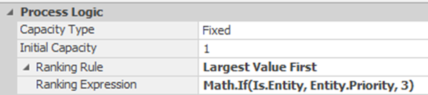
Figure 8.45: Setting Priority Based on Entity and Model
8.7.13 Save the model and rerun the experiment.
8.7.14 There does not seem to be any difference in time when we prioritized the applicants at each of the servers. Let’s add a dynamic label to the entities to display the priority value and see if the model is working as predicted. Select the EntApplicant ModelEntity and set the Dynamic Label Text property under the Animation section to display the priority as seen in Figure 8.46.
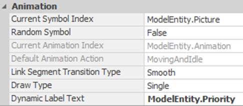
Figure 8.46: Adding a Dynamic Label that Moves with the Entity
8.7.15 Run the model and observe the output buffer of the SrvRegistration around the 9:30 am time frame.
8.7.16 The problem is there are three servers that have their own separate sorted queues when we really want one queue feeding those three servers to be sorted. The issue doesn’t happen in the other areas, as the entities are all in the same queue and sorted properly. To fix the issue, insert a Resource named ResTests with a capacity of three, and the Ranking Rule is set accordingly to act as this single queue. Also, select the ResTests and add the Allocation Queue from the Draw Queue in the Attached Animation section.

Figure 8.47: Adding a Resource to Act as Single Queue Feeding Three Servers
8.7.17 Next, we need to seize the new ResTests once the applicants enter the output node of the SrvRegistration as they try to get service at testing. Select the output node of SrvRegistration (i.e., Output@SrvRegistration) and add an Entered Add-On Process Trigger, as seen in Figure 8.48. The ResTests will determine which applicant to serve next and allow the applicant to move on to the testers.
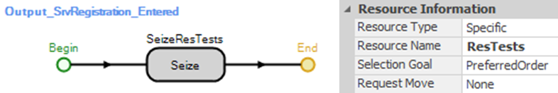
Figure 8.48: Seizing the ResTests in the Output Node of the SrvRegistration
8.7.18 Once the entity finishes the testing, we need to release the RestTests. Insert a Release step in the ProcessDataEntry right after the status is updated, as seen in Figure 8.49.
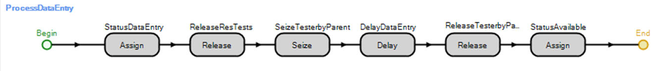
Figure 8.49: Releasing the ResTests After Finishing Testing
8.7.19 Save and run the model, observing whether or not the applicants are being ranked correctly now.
8.7.20 Next, rerun the experiment.
8.7.21 The applicants are now being processed correctly. However, on further reflection, if a walk-in applicant has been in the system for more than 30 minutes, they should be given greater consideration/priority. Because the time in the system changes while the applicant is waiting in the input buffer, the static Ranking Rule property cannot be used as it orders the queue as the entities enter the queue and are not reordered later. On the other hand, the Dynamic Selection Rule is evaluated each time the Server capacity becomes available in order to choose the next applicant. Select the SrvRegistration, SrvDrivingTest, and SrvPicture Server objects and specify the “Largest Value First” as the rule as seen in Figure 8.50 with the Value Expression equal to (Candidate.Entity.Priority==2) || (Candidate.Entity.TimeInSystem > MaxWaitTIme).
The expression will evaluate to either one (i.e., if the entity is a scheduled applicant or the entity has been in the system ½ hour) or zero otherwise.112 Repeat for the ResTests Resource object.

Figure 8.50: Specifying the Selection Rule to Prioritize Scheduled Applicants and Walk-ins
8.8 Controlling the Simulation Replication Length
The number of applicants that seem to be in the system at the end of the 7.5 hours that the DMV is open is of concern. After more discussion with the DMV personnel, you realize that the office closes at 4:30 pm, but the people stay until the last applicant is served. It is easy to run the simulation for exactly 7.5 hours using the “Run Setup” section of the “Run” tab. However, we need the simulation to stop after serving the last person. This concern raises two modeling issues. First, how do we stop the arrivals after 4:30 pm? Second, how do we stop the simulation run after the last person has left the system? There are various ways to stop applicants' arrival after 7.5 hours. For example, we could transfer them to a sink if the current time is after 4:30 pm (i.e., using selection weights on the paths). Another way would be to create a Monitor that would cause a process to alter the interarrival time or the entities per arrival.
Note that the current ArrivalRateTable only has 15 time periods, representing 7.5 hours. If we extend the simulation run length beyond 7.5 hours, SIMIO will cycle back to the beginning of the table, repeating the values because they are relative offset values. The only way to force zeros is to extend the arrival table to contain 24 items (i.e., 12 hours) and set the remaining values to zero. A direct method to stop the arrivals is to use the “Stopping Conditions” within the Source, which turns off arrivals based on either specifying a maximum number of arrivals113, some maximum time, or some stoppage event.
8.8.1 Select the SrcArrive Source and specify the Maximum Time property with a value of 7.5 under the Stopping Conditions section.
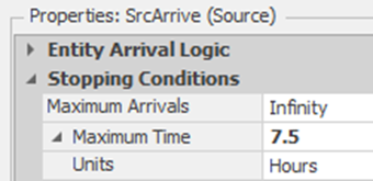
Figure 8.51: Stopping Arrivals after 4:30 pm
8.8.2 Set the run length to 12 hours and then run the model. You will notice that the applicants stop arriving at 4:30 pm, but the simulation continues displaying services (i.e., failures). A simulation run can be stopped using the End Run step. However, this step needs to be invoked under two conditions: (1) at 4:30 pm, in case no one is in the system, and (2) the more likely case when the last applicant is served after 4:30 pm.
8.8.3 Let’s first consider the case that the last applicant finishes after 4:30 pm when no more arrivals are permitted. Applicants exit the system through one of the three sink objects. So, at each of the sinks, we need to test whether this entity is the last applicant in the system and if it is after 7.5 hours. We will first create a general process.
- Go to the “Processes” tab and click on the “Create Process” button, naming the new process TimeToStop. Add a Decide and End Run step as in Figure 8.52.
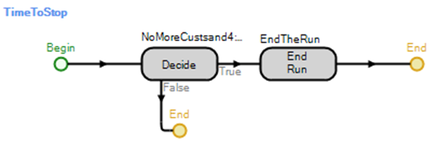
Figure 8.52: Check Last Applicant and End Run
- The Decide step is “ConditionBased” on the following expression.
(EntApplicant.Population.NumberInSystem <= 1) && (Run.TimeNow >= 7.5)
This expression states that we will stop the replication if the current applicant being destroyed is the last applicant in the system and the simulation time is greater than or equal to 7.5 hours.
8.8.4 Select the “Destroying Entity” add-in process trigger property for each of the three sinks and specify the TimeToStop process for each.
8.8.5 Within the Run→Run Setup, arbitrarily set the Run Length to 12 hours to be sure the simulation length does not end the run.
8.8.7 If you make multiple replications, each replication will stop at a different time. Output statistics are appropriate for collecting statistics on the time the replications stop. Note that output statistics only collect one observation for each replication at the end of the run. Such statistics will allow us to determine how long the office stays open on average. From the Definitions→Elements section, insert a new Output Statistic named OutStatOfficeCloses with the expression Run.TimeNow and set the UnitType to “Time” and Units to “Hours.”
8.8.8 Multiple replications of the model need to be executed to determine how long the office is open. From the “Project Home” tab, insert a new experiment named ExpOfficeCloses.
8.8.10 You need to add a response to evaluate each experiment scenario. Under the “Experiment” section, click the Add Response button to insert a response named TimeAfterClosing, which has an expression for the OutStatOfficeCloses.Value-7.5. This will indicate when the simulation ended minus the 7.5 hours representing the amount of time over the normal day (see Figure 8.53).114
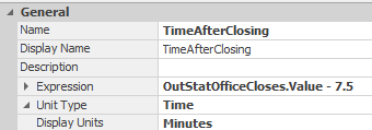
Figure 8.53: Specifying a Response for the Experiment
8.8.11 Save the project and execute the experiment, and from the Pivot grid, answer the following questions.
8.8.12 Click on the “Response Results” tab to see the (SIMIO Measure of Risk \& Error (SMORE) plot for the one response as seen in Figure 8.54. SMORE plots allow you to visualize the output response. It concisely displays the minimum, maximum, mean, median, lower, and upper percentiles,115 as well as the confidence intervals of the mean and the lower and upper percentiles. The histogram of values is also displayed because the “Histogram” button is pushed.
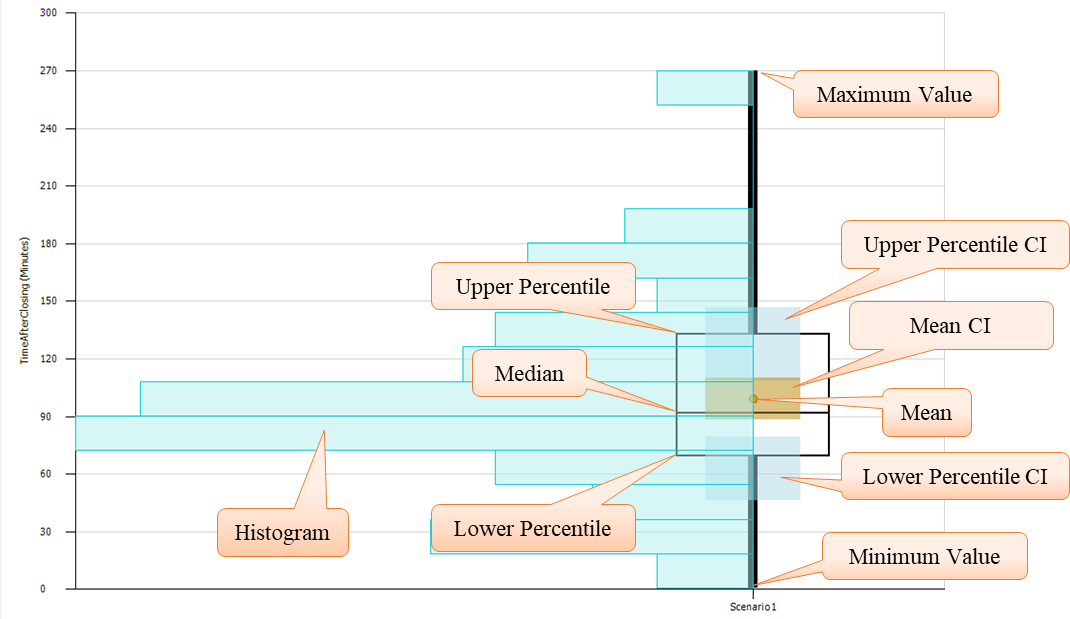
Figure 8.54: SMORE Plot with Histogram for the Additional Time the Office is Open
8.8.12.1 Based on the SMORE plot and its “Raw Data,” what are the mean and the 95% confidence intervals of the additional time office is open?
_______________________________________________
8.8.12.2 What are the lower and upper percentiles and their values?
_______________________________________________
8.8.12.3 What is the maximum additional time spent in the office, and does that make sense?
_______________________________________________
There are occasions when the maximum additional time spent is 7.5 hours (450 minutes) either via the SMORE plot or the results in the Pivot Grid. The simulation does not stop until the 15-hour run length is reached. Note an observation in a sink must occur before the stopping condition is checked.
8.8.13 In this situation, the last applicant leaves the system, but the current time is still less than 7.5 hours; therefore, the stopping condition is not invoked. The previous stopping method assumes that there would always be applicants in the system at 4:00 pm. The model needs to check to see if there are zero applicants at closing. Return to the Model, insert a new Timer element named TimerToStop from the Definitions→Elements section, and set the Time Interval property to 7.5 hours116.
8.8.14 In the Processes tab, insert a new process named StoppingSimulation, which utilizes the TimertoStop event as its Triggering Event Name property and the Triggering Event Condition, as seen in Figure 8.55. The process will only run when the event occurs if the triggering event condition is also true.
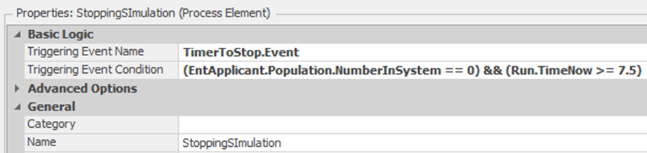
Figure 8.55: Specifying a New Process to be Executed when the Timer Fires
8.8.15 Insert the End Run step, which will stop the simulation run as soon as the step is executed, as shown in Figure 8.56.

Figure 8.56: Stopping Simulation at Time 7.5 hours Process
8.8.16 Save the model and rerun the experiment, looking at the “Response Results” again.
8.8.16.1 On average, how long does the office stay open past the 7.5 hours?
_______________________________________________
8.8.16.2 What is the maximum additional time spent in the office, and does that make sense?
_______________________________________________
8.9 Commentary
- In Figure 8.39, the appointment schedule was designated using absolute dates and times. Internally, SIMIO converts the table into a time offset table based on the simulation starting date and time. One can also specify the appointment table directly as time offsets, as seen in Figure 8.57 Which represents the exact same table. The column type must be a numeric or an expression general property.
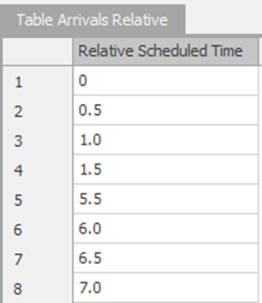
Figure 8.57: Appointment Table Using Time Offsets
The Process Type property can be changed to handle more complicate sequences rather just a “Specific Time” and will be explored in a later chapter.↩︎
A problem often arises when a client/boss sees the animated model not conforming exactly like the real system. Some people (naively) equate the “quality” of the model with the quality of the animation. Sometimes you are forced into animation details that have little to do with performance measures.↩︎
Note, different Sinks will be used to separate the statistics for those that fail test versus not. From an animation standpoint, one can put the three Sinks on top of one another to demonstrate the applicants leaving the same door so it visually looks correct.↩︎
Switch to 3-D mode to color the entire entity widget.↩︎
We have a strong preference for processes over the specifications in objects (e.g., the table, state, tally properties), since processes give use the most flexibility in specifying and re-specifying these additions to the model.↩︎
It is convenient to use the Secondary Resources when you don’t need the flexibility of the add-on processes. Resources for Processing does both the seizing and releasing of the resources.↩︎
By default the capacity requested will only be one. You have more flexibility with the Seize step.↩︎
An Interrupt step can be used to model interrupts.↩︎
You can modify the existing resource object so it has capacity one and its Uptime Between Failures as Random.Exponential(120) minutes. Then copy the object three times and name them accordingly.↩︎
The Seize process step has the same issue of being able to seize from a single object.↩︎
Do not confuse the Selection Expression property with the Selection Condition which is used to include/filter candidate nodes.↩︎
Note the Candidate object has to be used to specify a wildcard like ‘*’. SIMIO will replace the Candidate object with the appropriate object from the list when determining the smallest value. Also, if there is a tie between nodes they will be selected in the order they were placed into the list.↩︎
The Contents queue of the InputBuffer Station is used to hold entities waiting to be processed by the Server.↩︎
The Contents queue of the Processing Station represents the location of the entities that are currently being processed by the Server.↩︎
The ! or Not operator can be used to take the complement of a variable (i.e., ! False would equal True).↩︎
Here “Available” is a string constant (arbitrarily chosen), not a numerical value.↩︎
Note we could have created three individual state variables (i.e., GStaTesterStatus1, GStaTesterStatus2, and GStaTesterStatus3) instead of the one variable that is a vector of size three.↩︎
One could shut down the path by changing the capacity or the direction to None or potentially cause the TransferNode Current Travel Capacity state variable to go to zero.↩︎
Note, the \&\& is for logical “And” such that we only select servers that have not failed and currently not processing someone.↩︎
From an animation standpoint, we would delete the input buffer queues of the testing stations, driving test, and picture area.↩︎
Note, you can build the table in Excel as it can be easier and then copy the table into SIMIO.↩︎
Negative times mean the entity is early for their appointment, whereas positive number implies they are late.↩︎
The Priority assignment could be done within the process SrcArrive_CreatedEntity.↩︎
If there is a tie (i.e., multiple entities have the same value), they are ordered based on First in First out rule.↩︎
Note that this is the number of total “arrival events” and not the total number of entities arriving. One arrival event may yield more than one entity arriving.↩︎
Note we could have made the Output statistic expression be Run.TimeNow – 7.5 instead.↩︎
By default it is the 25th and 75th percentiles which can be changed on the Experiment properties along with the default 95% confidence interval.↩︎
One timer event will occur at 0.0 since the Time Offset is 0.0, but it won’t affect the simulation in this case.↩︎