Simulation Modeling with Simio - 6th Edition
Chapter
11
Simulation Output Analysis
You have carefully created a model and paid close attention to the present operational system. Your model produces appropriate performance measures. You may have done some considerable re-modeling as you learned more about the system being modeled and its important aspects. You have been concerned about modeling errors, so you checked your model often and verified it is working the way you want. Furthermore, you have addressed the question of model validity by checking the simulated performance measures against actual results. Through all your efforts, you have been thinking about ways to improve the system performance and have an accumulated set of alternative scenarios you want to try. You are now satisfied that you can begin to examine these alternative scenarios and begin the process of developing recommendations.
The simulation model produces outputs, but we know they are sets of random variables. But how do we best understand these results? We can generate averages of observed outputs, but these averages exhibit variation. Can we simply make multiple replications of our model, create confidence intervals, and draw conclusions?
11.1 What Can Go Wrong?
There are two overriding statistical issues that should concern us. The first is bias in our estimates, which are potentially wrong estimates. The second is the “independence and identicalness” assumptions, which plague us when calculating measures of variability and ultimately comparing systems.
Bias
Perhaps the biggest concern is the potential “bias” in our computed averages. Bias means that we computed a value that is systematically different than the performance measure of interest. In other words, we may be computing a value that simply isn’t the value of interest. Bias can occur in our method of calculation, but it is more likely in the values being used. For instance, consider the computation of the average waiting time in the queue of the ice cream store. Now, we know that the simulation starts “empty and idle,” so the early waiting times will be considerably smaller than those during the day. In fact, the expected waiting time changes throughout the day. Since the arrival process uses a time-varying arrival, the waiting times grow and shrink with a strong influence from the arrival rate. Other statistics, like resource utilization, will vary as well.
Bias may or may not be a problem. If we need to know the waiting time, say during the busiest time in the ice cream store, computing the waiting time during the entire day will clearly underestimate that waiting time. In such a case, we need to collect our own statistics during the periods of interest. On the other hand, an overall average waiting time computed over the whole day can be useful. While it may underestimate our intuition about the congestion, it is a systematic and consistent computation that can be useful in comparing alternative scenarios. Because the waiting time will be computed in the same manner in all scenarios, the observed improvement or deterioration will be “relatively” correct. In other words, our absolute estimate of waiting times may be an underestimate, but that same degree of underestimation will be present in all scenarios explored.
This idea that relative differences are the important perspective allows us to use simulation models that underestimate many performance measures simply because all the “small” factors that impact the performance measure are being ignored. For instance, our simulation model may only account for 50% of a resource’s duties when we know their workload is closer to 80%. But because all our scenarios ignore those same small factors (e.g., meetings, breaks, interruptions), if we find a scenario that enhances the resource to 60% utilization, then we believe that the base utilization of the resource will be increased by 10% by employing this scenario. So, the recommendation here is to use a relative difference perspective rather than an absolute perspective when possible.
Independent and Identically Distributed
In order to measure variability associated with any simulation output, one needs data to be independent and identically distributed (IID). The reason is that the confidence interval computation for an expected value is based on the central limit theorem, which allows us to compute the standard deviation of the mean from the standard deviation of the observation. Unfortunately, variability is present in almost all our simulation output, so we had to “construct” IID observations. Early in our study of simulation, we recognized that the observations within a single replication do not satisfy the IID requirement. So, we rejected the observed waiting times within a simulation replication as unsuitable for estimating the variance of an expected value. Instead, we compute the replication average as an observation, which works for most of the cases of interest.
There are a couple of situations where getting the IID observations may be a cause for concern. One case occurs when a simulation replication takes a very long time. It becomes very costly (in terms of computer time) to run all of the appropriate replications needed. A second case is when the simulation starts from, for example, empty and idle, and there is a lengthy period when the performance measures are poorly estimated due to the startup of the simulation. In both cases, using replications (i.e., one observation per replication) becomes problematic since we have limited opportunity to do many replications.
11.2 Types of Simulation Analyses
There are two general types of simulation analyses: terminating and steady-state. A terminating simulation typically models a terminating system that has a natural opening and closing. The ice cream store is a good example because it opens empty and idle in the morning and then closes in the afternoon, sometimes after the last customer is served. Terminating simulations are characterized by their opening and closing. Thus, any performance measures computed implicitly depend on how the simulation starts and stops. One replication is generally the time between the opening and closing. A terminating simulation is sometimes called a “transient” simulation because its state is constantly changing throughout the replication. Although bias in the estimates of the averages may occur because of the changing state, the estimation of variance is facilitated by the use of replications.
11.2.0.1 What is an example of a simulation that should be examined as a terminating simulation?
_______________________________________________
A steady-state simulation has no “natural” opening or closing. In a steady-state simulation, we want our performance measures to be independent of how we started or stopped the simulation. In other words, we want a kind of long-term average for the expectations. However, while there is considerable appeal for performance measures that are independent of starting and stopping, how to obtain such a simulation is not clear. There are two fundamental problems. The first is how to eliminate the effects of startup or warmup. The influence of the way the simulation starts can extend far into the simulation. The second problem is how long a replication should last since there is no natural stopping state. Neither of these problems can be easily answered, so the tendency is to resort to “rules of thumb” that give some general guidance but for which there is limited theory.
11.3 Output Analysis
To provide a context for an output analysis, re-consider the work cell problem of Chapter 5, section 6. Recall that this problem is a manufacturing cell consisting of three workstations (i.e., A, B, C) through which four-part types are processed. The parts have their own sequences, and processing times depend on the part type and the station visited. We defined two statistics of interest: a “state statistic” on the number of Part type 3’s in the system during the simulation and a “tally statistic” on the time Part type 3’s are in the system.
Very little analysis of the problem was undertaken. We ran the simulation (interactively) for 40 hours and examined the output. The average number of Part type 3’s in the system was 0.40 parts, and the average time for Part type 3’s in the system was 0.26 hours. At that time, our focus was on the construction of the model, not necessarily the interpretation of the output, which we will explore now.
Since we have more experience with simulation output, we may be considering a SIMIO experiment and making multiple replications. By making multiple replications, we obtain an estimate of the variability associated with the observed averages and could compute a confidence interval. But before doing that analysis, let’s think about our simulation intent. How do we want to use the output from the simulation? Do we want to say something about the “short-term” or the “long-term” outcomes? We probably chose a 40-hour simulation length because it represents a “week’s worth” of work. However, we also used the default “empty and idle” state for the start of the week. Is that representative of a real week? If the answer is yes, then we can make multiple replications and create confidence intervals for our output measures.
11.3.0.1 In your judgment, how likely are you interested in one week’s statistics being empty and idle at the beginning of the week?
_______________________________________________
By doing replications, we should obtain approximate IID observations, but a more fundamental concern is bias. We have two sources of bias. The first is the “initialization” or “warm up.” Starting empty and idle certainly affects our statistics. The second is whether the 40 hours is sufficient time to observe the system. To limit our discussion, let’s focus primarily on the two user-defined statistics: the number of Part type 3’s in the system during the simulation and the time Part type 3’s are in the system.
Initialization Bias
When we describe the initialization bias, we often use the term “warm up,” implying that the simulation output goes through a phase change like a car that needs to warm up in cold weather before turning on the heater. We think of a “transient phase” followed by a transition to the “steady-state phase.” And usually, the steady-state phase interests us since it represents the “long-term” perspective.
Three “obvious” ways to deal with the initialization bias are: (1) ignore it, trusting that you have enough “good” statistical contributions from the steady-state phase that the “poor” statistics at the beginning (during the transient period) are completely diluted, (2) “load” your system with entities at the beginning of the simulation so that the transition to steady-state behavior occurs early, and (3) after a while (i.e., warm up period), clear (truncate) the statistics in an attempt to clean out the transient statistics so they can no longer influence the statistics collection.
The problem with ignoring the presence of the transient statistics is that their influence on the final statistics is really unknown. The problem with loading the system with entities is that we don’t know where the loading should take place and furthermore, we don’t know that our loading really hastens the transition to steady-state. Finally, the problem with deleting statistics is that we delete “good” as well as “bad” statistics and simulation observations are important and usually somewhat hard to obtain. So, let’s consider a more thorough examination of initialization bias in the context of the work cell problem.
11.3.1 Open up the simulation from Chapter 5, section 6. For comparison purposes, run the model interactively for 40 hours.
11.3.2 Add a SIMIO Experiment, specifying ten replications, each replication being 40 hours. We will also use these results for comparison.
11.3.2.1 What is the 95% confidence interval on the average number of parts of type three in the system during the 40 hours?
_______________________________________________
11.3.2.2 What is the 95% confidence interval on the average time parts of type three are in the system during the 40 hours?
_______________________________________________
11.3.3 Next, let’s add some plots of the two user-statistics so we can visualize the change in these over time due to the initialization bias. Keep in mind this simulation starts empty and idle. Add two Animation Plots from the Animation tab: one for the number of parts of type three in the system and the second for the time parts of type three are in the system. Figure 11.1 shows the specifications for the average number of part type three in the system. Figure 11.2 shows the specifications for the average time part type 3 is in the system.
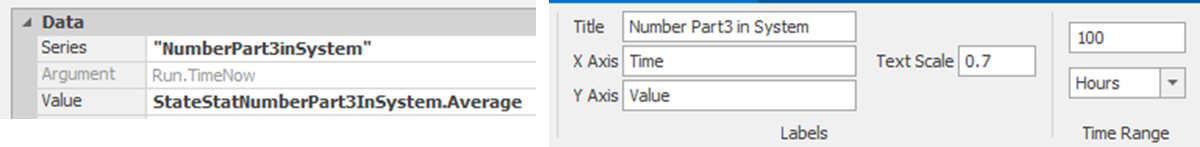
Figure 11.1: Animation Plot for Average Number of Part Type 3 in System
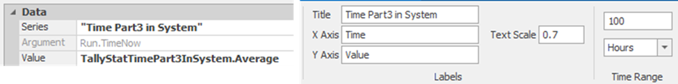
Figure 11.2: Animation Plot for Average Time Part Type 3 in System
11.3.4 Be sure that the Time Range on the plots is 100 hours so we have enough time to see the changes.
11.3.5 Change the run length of the simulation to 100 hours and, run the simulation interactively (set the speed factor to 1000) and observe the plots.
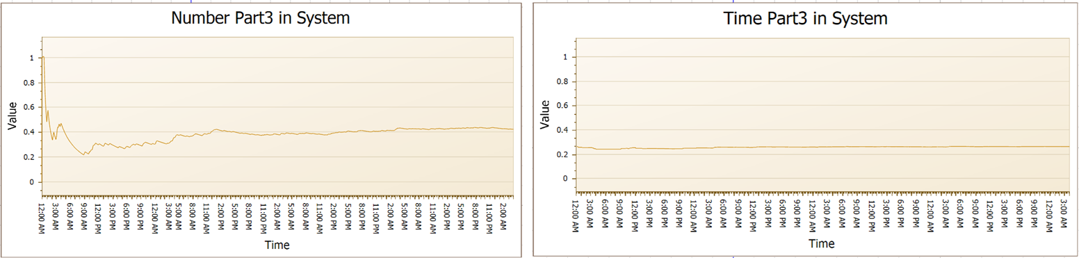
Figure 11.3: Average Number and Time in System
11.3.6 Notice how the number in system plot changes rather markedly during the first 50 hours, while the time in system plot doesn’t change much.
11.3.6.1 During the initial 50 hours, how long does the transient period seem to last (recall this is the time during which the behavior is erratic)?
_______________________________________________
11.3.6.2 After the transient period, there is a period of transition as the state of the statistics moves from being highly unstable to becoming stable. How long do you think this transition period lasts?
_______________________________________________
11.3.6.3 How are the animation plots changing during the last 50 hours?
_______________________________________________
When these plots stabilize, we say the statistics are in steady-state. Notice that we talk about the statistics, not the system because it’s the statistics that interest us, even though it’s the system that is changing.
11.3.7 We have seen only one replication during the 100-hour simulation. Under the Advanced Options within the Run Setup section of the Run tab, click on Randomness and select the Replication Number option. Set the replication number to “2” and re-run the 100-hour simulation. Now, the time in the system continues to be relatively stable, while the number in the system shows a different transient behavior. Figure 11.4 shows the average number of part type three’s in the system during the first 100 hours.
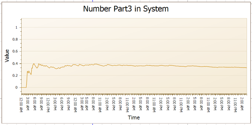
Figure 11.4: Replication 2 Average Number Part 3 in System
11.3.7.1 How does the transient phase in Replication 2 for the average number of part 3 in the system differ from the one for Replication 1 (which is shown in Figure 11.3)?
_______________________________________________
11.3.8 Now, continue to change the replication number and interactively simulate, observing the behavior of the average number of part 3’s in the system during the first 50 hours. Figure 11.5 shows the results for replications 3, 4, and 5. We focus on number in system, but be sure to look at the time in system also.

Figure 11.5: Replications 3, 4, and 5 Average Number of Part Type 3 in System
11.3.9 With these five replications, we can see a range of behaviors at the beginning of the simulation. In all cases, the statistics appear to converge to a common steady-state value, but there was a consistent transient period during which there was no consistent behavior.
11.3.10 Now simulate Replication 5 for 40 hours interactively and compare to Step 1.
11.3.10.1 What is the average number of parts of type three in the system during the 40 hours?
_______________________________________________
11.3.11 While the differences are probably not important in this case, you can see that they may be in other cases. In any case, our simulation would benefit by eliminating the initialization bias. Now, the question is, how large should the warmup be? Clearly, we want to eliminate the transient period, which, after observing five different replications, lasts for about 20 hours. The transition period still shows some effect, but we don’t want to throw away observations unless we think they are really bad. So, let’s make the warmup period 15 hours.
Replication Length
Now, as a rule of thumb, we do not want the warmup period to exceed 10-20% of the length of a replication. In fact, if time permits, 5% would be a target.
11.3.12 So, let’s run the simulation experiment with a run length of 150 hours with a warmup of 15 hours with a total of 10 replications.
11.3.12.1 What is the 95% confidence interval on the average number of parts of type three in the system?
_______________________________________________
11.3.12.2 What is the 95% confidence interval on the average time parts of type three are in the system?
_______________________________________________
11.3.12.3 How do these confidence intervals compare to the ones from Step 2 previously?
_______________________________________________
In summary, removing the initialization bias by using the warmup period is important. However, you should look at several replications of the warmup period in order to understand the range of behavior. Also, you need to examine all the statistics of interest so your warmup covers the largest transient behavior. With the warmup period established, be sure that the warmup period is less than 20% of the replication length. It is generally a good rule to multiply the warmup period by 10 to obtain the replication length. Use a multiplier of 20 if your model runs quickly enough.
11.4 Automatic Batching of Output
To obtain our previous confidence interval, we simulated (150 hours * 10 replications) for a total of 1500 hours. Of that total, we used 450 hours for the warmup. Although this small problem runs through that simulation time rather quickly, a larger problem may take hours of computer time to provide such a confidence interval. So, we may be interested in obtaining a confidence interval in less time. We “wasted” many observations during warmup and created fairly lengthy simulation replications.
An alternative to replications is employing a method known as “batch means.” Using batch means, we attempt to create IID observations within one long replication. Since only one run of the simulation is used, we only lose the warmup observations once, and we are able to invest our simulation effort in one long run rather than several. Hopefully, all this means that we save simulation time. The batch means method creates “batches” of observations for which the average for the batches satisfies our IID requirement. For example, the time-persistent statistics (state statistics), like the number in the system, may have a mean computed every 25 hours if the means from every 25 hours appear to be IID. For observations-based statistics (tally statistics), we might compute an average waiting time for every 50 customers if the means from every 50 customers appear to be IID. The 25 hours for state statistics and the 50 customers for tally statistics are called the “batch size.” There will be two batch sizes: one for state statistics and one for tally statistics. The number of batches created during the simulation corresponds to the number of observations when computing a confidence interval.
SIMIO will automatically employ a version of batch means to compute a confidence interval when: (1) user statistics are defined, and (2) an SIMIO experiment with one replication is employed. The only SIMIO-defined statistics that will be automatically batched are the sink node statistics.
11.4.1 Use the simulation model from the previous section. Change the number of required replications to one. Leave the warmup at 15 hours and leave the replication length at 150 hours.
11.4.2 When you execute the simulation, you will see a new row called “HalfWidth” in the two user-defined statistics for the average number of part type 3 in the system and the average time part type 3 is in the system. You will also see that new row in the SnkPartsLeave statistics on flowtime. The output for the two user-defined statistics is shown in Figure 11.6.
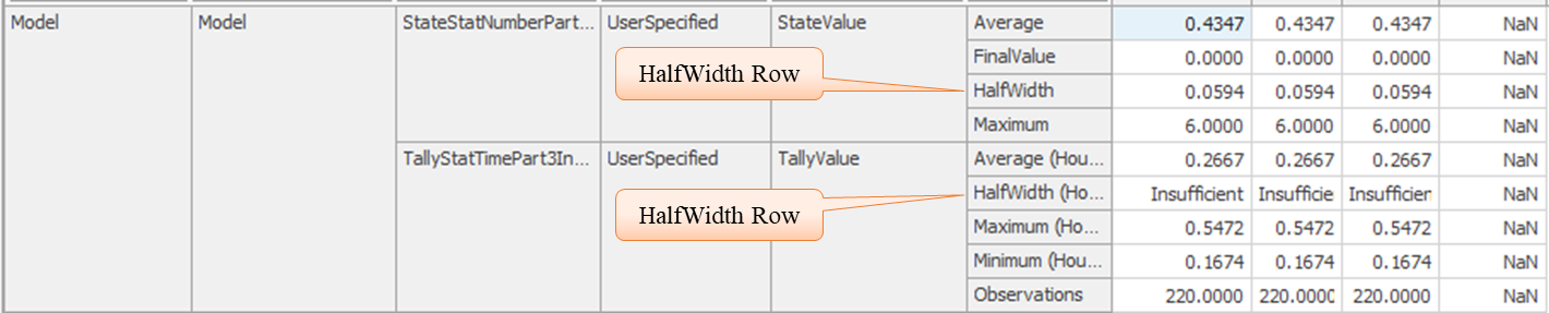
Figure 11.6: Output for User-Defined Statistics
11.4.3 In the case of the time in system we see an “Insufficient,” meaning we have run the simulation long enough for SIMIO to obtain enough batches to compute a confidence interval. It is also possible to get a “Correlated” message meaning that the obtained batches do not satisfy the IID requirement. Figure 11.7 is an example of obtaining this message.

Figure 11.7: Example of Correlated Batch Means
11.4.4 Now, change the replication length to 300 hours, which is twice the length of the earlier replications.
11.4.4.2 What is the 95% confidence interval on the average number of parts of type 3 in the system?
_______________________________________________
11.4.4.3 What is the 95% confidence interval on the average time parts of type 3 are in the system?
_______________________________________________
11.4.4.4 How do these confidence intervals compare to the ones from Section 3 previously?
_______________________________________________
The automatic batching of statistics by SIMIO was able to produce a “legitimate” confidence interval with only 300 hours of simulation, as opposed to the 1500 hours previously. When using automatic batching, we still needed the warmup analysis.
11.5 Algorithms used in SIMIO Batch Means Method
SIMIO automatically attempts to compute a confidence interval via a batch means method for only the user-defined tally and state statistics (the only exception is that the batch means method is also applied to sink statistics) for a SIMIO Experiment having only one replication. It displays the results in the output in the row called “HalfWidth,” which is one-half the confidence interval. It can fail to make the computation if it believes there is insufficient data or if the batched data remains correlated. SIMIO does not include data obtained during the Warmup Period specified in the Experiment.
SIMIO’s batching method is done “on the fly,” meaning the batches are formed during the simulation. Thus batches can be enlarged but not re-batched.
Minimum Sufficient Data
- For a Tally statistic, SIMIO requires a minimum of 320 observations
- For a State statistic, there must be at least 320 changes in the variable during at least five units of simulated time.
- For statistics that do not satisfy this minimum requirement, the half width is labeled “Insufficient.”
Forming Batches
- Form 20 batch means
- A Tally batch is the mean of 16 consecutive observations
- A State batch will be the time average over 0.25 time units
- Continue forming batches until there are 40 batches
- At 40 batches, the batch size is doubled (each batch is “twice as big”), and the number of batches is reduced to 20
- Continue this procedure as long as the simulation runs. Notice that the number of batches will be between 20 and 39
Test for Correlation
- SIMIO uses VonNeuman’s Test147 on the final set of batches to determine if the assumption of independence can be justified.
- If the test fails, the half-width is labeled “Correlated.”
- If the test passes, the half-width is computed and displayed.
Cautions
The SIMIO batch means the method is only for steady-state analysis – it should be ignored entirely for terminating systems. There is no automatic determination of the warmup period. All rules for collecting batches are somewhat arbitrary, so some care needs to be exercised when using them.
11.6 Input Analysis
It may seem strange to include “input analysis” in a chapter devoted to “output analysis,” but it must be remembered that the analysis of the input is based on the behavior of the output. SIMIO provides two input data analyses: (1) Response Sensitivity Analysis and (2) Sample Size Error Analysis. Both analyses require that at least one of your inputs be an Input Parameter and that you have defined at least one Experiment Response. Although we briefly introduced response sensitivity analysis previously, we will describe it as well as the sample size error analysis within the same context, namely the work cell problem used throughout this chapter.
Recall that “input parameters” are defined from the “Data” window tab in three possible ways: (1) through a Distribution you hypothesized, (2) with a Table of observations that you have collected, and (3) using a SIMIO Expression. Any defined input parameter can be used anywhere in your model, and various objects can reference the same input parameter. Using distributions has the advantage that SIMIO will provide you with a histogram based on 10,000 samples to show you what that distribution looks like.
11.6.2 Rename the model state variable to GStaNumberInSystem. Modify the two user-defined statistics so we have some possible responses for experimentation. Call the state statistic StateStatNumberInSystem and the tally statistic TallyStatTimeInSystem. Be sure that the state statistic references the GStaNumberInSystem state variable and that the tally statistic has Time as the Unit Type.
11.6.3 Fix the State Assignment at the SrcParts and the SnkPartsLeave so that GStaNumberInSystem is always incremented (add one) at the source and decremented (subtract one) at the sink. Modify the Tally Statistics collection at the Input@SnkPartsLeave to correspond to Figure 11.8.
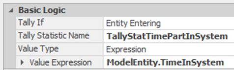
Figure 11.8: Tally All Entities Time in System
11.6.4 Next, we need to create the input parameters, which will correspond to, in this case, all the distributions used in the model. These are created by specifying a “Distribution” with the Input Parameters section from the “Data” Tab. Make sure to change the Unit Type property to “Time” and specify minutes. Figure 11.9 shows the inputs, and these are the same as the SequencePart table.
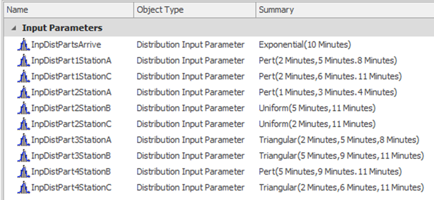
Figure 11.9: Definition of Input Parameters
11.6.6 Also, substitute the appropriate input distribution into the SequencePart Data Table for each of the ProcessingTimes values, as seen in the partial view of the table in Figure 11.10.
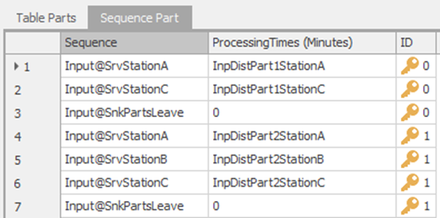
Figure 11.10: Partial View of the Sequence Part Table using the New Input Distributions
11.6.7 Next, select the Experiment and add two experiment responses, as shown in Figure 11.11.
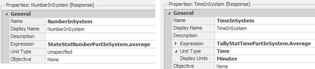
Figure 11.11: Experiment Responses for Number and Time in System
11.6.8 Run the experiment with a Warmup Period of 15 hours and a run length of 150 hours with 20 replications, which will be used as a base reference for the results.
11.6.8.1 What did you get for the 95% confidence interval on the average number in the system?
_______________________________________________
11.6.8.2 What did you get for the 95% confidence interval for the average time in the system?
_______________________________________________
Response Sensitivity Analysis
The response sensitivity analysis measures how each response is affected by changes in the input parameters. It will be computed for each scenario in the experiment. A linear regression relates each input parameter to each response, so the number of replications must be greater than the number of input parameters.
11.6.9 Our prior model had ten input parameters, and we used 20 replications. Select the Input Analysis tab and then the Response Sensitivity icon and run the model (it may be necessary to Reset it first). The results of the sensitivity analyses are shown in a Tornado Chart, a Bar Chart, and a Pie Chart. The raw data for each of the regressions are also available.
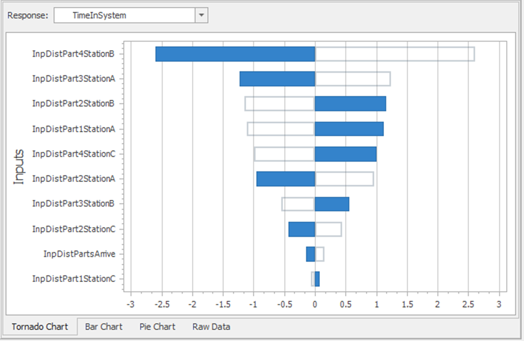
Figure 11.12: Tornado Chart for Time in System
11.6.10 Refer to the Tornado Chart in Figure 11.12 and pass your cursor over the bars. If an input parameter has a negative coefficient, then when it is increased, it reduces the response. If the input parameter has a positive coefficient, then when it is increased, it increases the response. The magnitude of the coefficient determines its importance relative to the other input parameters.
11.6.10.1 What input parameter will reduce the time in system the most when its distribution is increased?
_______________________________________________
11.6.10.2 What input parameter will increase the time in system the most when its distribution is increased?
_______________________________________________
11.6.10.3 What input parameter reduces the number in system the most when its distribution is increased?
_______________________________________________
11.6.10.4 What input parameter increases the number in system the most when its distribution is increased?
_______________________________________________
11.6.10.6 What is the primary value of the pie chart relative to the sensitivity analysis?
_______________________________________________
Sample Size Error Analysis
The sample size error analysis attempts to assess the uncertainty in the responses relative to the uncertainty in the experiment and the uncertainty in the input parameter data. To perform this analysis, it is assumed that the input parameters were estimated from collected data samples. In other words, you have a record of observations you used for a given input parameter estimation (or distribution fitting).
11.6.11 Pretend you have collected data for the input parameter estimation. From the Mode and the Input Parameters on the “Data” tab, select a defined input parameter. Change the Number of Data Samples property according to Table 11.1 and be sure that the Include Sample Size Error Analysis property is True.
| Input Parameter | Data Samples |
|---|---|
| DistPartsArrive | 125 |
| DistPart1StationA | 85 |
| DistPart1StationC | 85 |
| DistPart2StationA | 100 |
| DistPart2StationB | 100 |
| DistPart2StationC | 100 |
| DistPart3StationA | 60 |
| DistPart3StationB | 60 |
| DistPart4StationB | 45 |
| DistPart4StationC | 45 |
11.6.12 Go to the Input Analysis tab within the Experiment. Select the Sample Size Error icon and run the analysis (after doing a Reset). This may take a little bit of time to complete.
11.6.14 The two important tabs are: (1) Contribution to Uncertainty and (2) Benefit of Additional Samples. Look first at the contribution to uncertainty, shown in Figure 11.13.
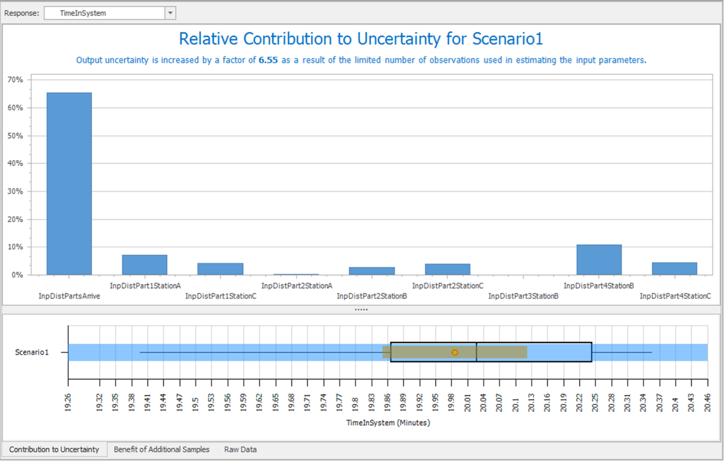
Figure 11.13: Uncertainty of Time In System
11.6.14.1 Which factor has the biggest impact on time in the system?
_______________________________________________
11.6.14.2 The SMORE plot illustrates the confidence interval for the mean (in tan), with the expanded half width due to input uncertainty in blue (and stated in the text). How much does the uncertainty in the input parameters “expand” the output uncertainty?
_______________________________________________
11.6.15 Next, look at the tab: Benefit of Additional Samples as shown in Figure 11.14.
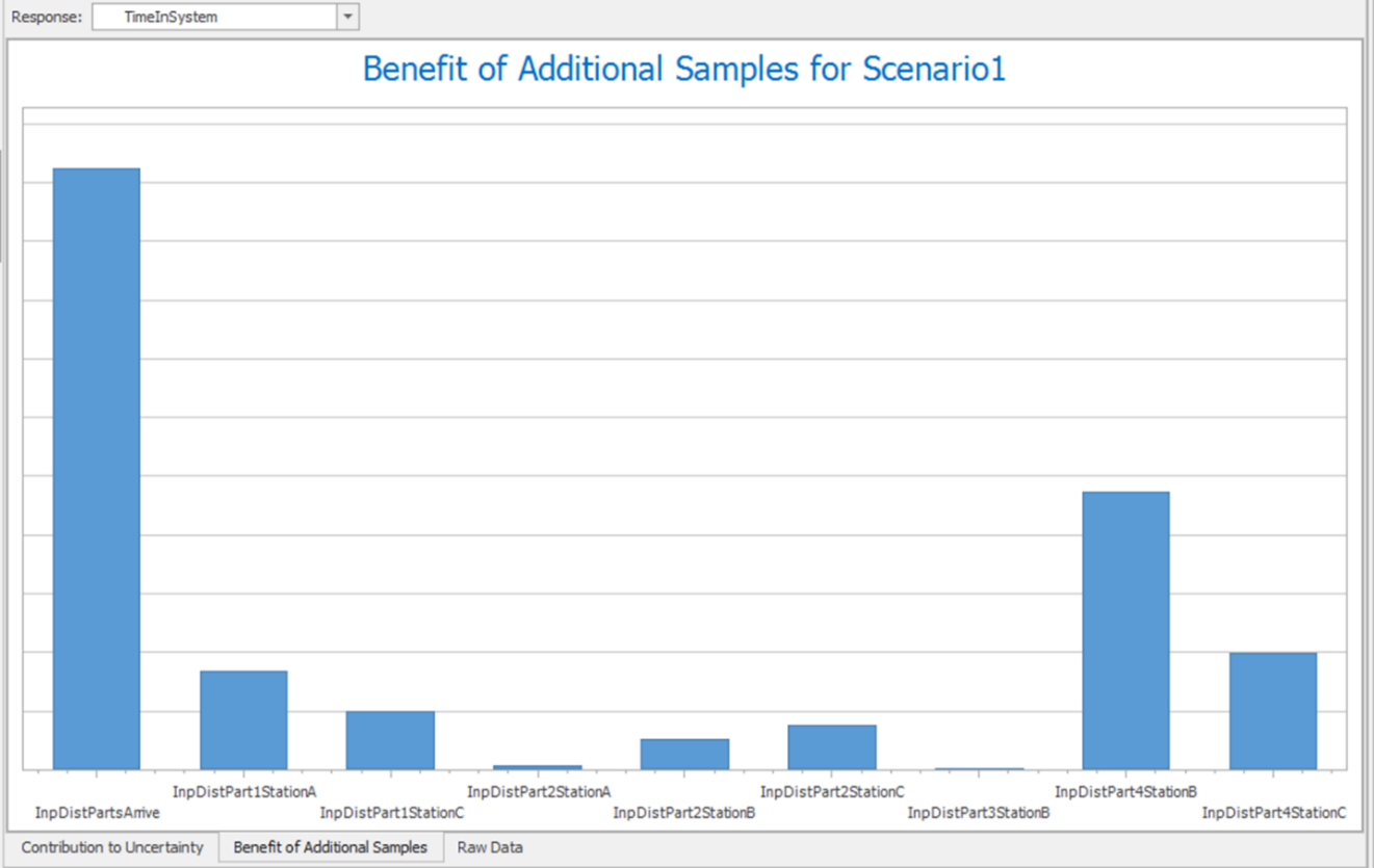
Figure 11.14: Benefit of Additional Samples
11.6.16 Go back to the Input Parameters and change the Number of Data Samples property for InpDistPartsArrive to 250. Next, repeat the sample size error analysis.
11.6.16.1 How does the Contribution to Uncertainty change?
_______________________________________________
11.7 Commentary
- Sometimes, the modeling effort consumes so much of a simulation project that the analysis of the model is almost overlooked. In particular, it is easy to forget that simulation output can be difficult to interpret and requires time and care. The issue of bias is often ignored, which can be a critical mistake.
- Replications permit the computation of confidence intervals, which are our best way to measure the mean and variance of the expected value.
- Our experience is that most simulations can be run quickly, which means that eliminating the warmup and replications becomes feasible even for steady-state simulations. However, some steady-state simulations take excessive computer time, so the idea of using batch means becomes attractive.
- The availability input analysis features in SIMIO should encourage you to consider the importance of the simulation inputs relative to your performance measures. You can judge the value of the various inputs and consider the amount of data collection devoted to their specification.
This is a statistical test of independence.↩︎