Simulation Modeling with Simio - 6th Edition
Chapter
12
Materials Handling
You may have already noticed a Vehicle object and a Conveyor path in the Standard Library. Perhaps the term “vehicle” already conjures up the idea of moving materials or people from place to place, and your intuition would be correct. The vehicle object can pick up and delivery entities which can be used to act as a forklift truck in a manufacturing operation, a human stock handler in a warehouse, a taxi cab for picking up and delivering people, as well as a bus, a train, or other type of people mover to move entities either individually or in a group. The Vehicle is an individual object whose routing is based on either “demand” or a “fixed path.” A conveyor in SIMIO, on the other hand, provides a continuous platform for conveying items or people. It can represent various industrial devices like gravity conveyors, belt conveyors, powered overhead conveyors, and even a power and free conveyor. Often, materials handling in the industry employs a variety of materials handling devices. A distinction among conveyors used by SIMIO is whether the conveyor “accumulates” or doesn’t (“non-accumulating). An accumulating conveyor allows entities to queue up at its end. A non-accumulating conveyor will stop when an entity gets to the end and won’t start up until that entity is removed.
A key to modeling materials handling problems in SIMIO is using the TransferNode and, to a lesser extent, the external OutputBuffer attached to many objects like the Source and the Server. The TransferNode (unlike the BasicNode) provides the “Transport Logic,” which means you can request a vehicle to move the entity to its next designation. If that transport device is not available, then the entity must wait. The TransferNode can be used alone, and entities can wait for pickup at that node, but they will not queue up in the usual fashion. For other objects, the OutputBuffer provides a place for the entities to wait for transportation.
12.1 Vehicles: Cart Transfer in Manufacturing Cell
We will reconsider the original problem of Chapter 5, whose layout and information are shown in Chapter 5, Figure 5.1. Recall that there are five different types of parts, each with its own routing through the manufacturing cell. However, we now learn that instead of leaving the system, parts actually have to be put on a cart and wheeled to the warehouse building 300 yards away (see Figure 5.9). The cart can carry a maximum of three parts and travels four feet per second. After the cart has finished dropping off parts, it will return to the pickup station for the next set of parts or wait until a part is ready to be taken. The cart does not have to be filled to be taken to the warehouse (i.e., it will carry one part if available).
12.1.1 Open up the last model from Chapter 5 and save it as chap12.1.
12.1.2 Delete the Connector between the Sink object and the prior BasicNode to facilitate a cart that takes the parts to the warehouse. Next, insert a TransferNode named TnodeCart between the SnkPartsLeave, as seen in Figure 12.1.
12.1.3 Select the Input@SnkPartsLeave and remove the Tally Statistics as Vehicles will be entering instead, and we do not want them contributing to the statistic. We could insert a Tally step in the Entered add-on process trigger to calculate the same statistics.
12.1.4 Connect the BasicNode to the TransferNode with a Path with a logical length of 10 yards. Finally, connect the TNodeCart TransferNode to the sink with a Path, ensuring its Type is set to “Bidirectional” so our cart can move in both directions. Set the path’s logical length to 300 yards.
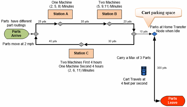
Figure 12.1: Adding a Vehicle to Carry Part to the Exit
12.1.5 Drag and drop a Vehicle object from the [Standard Library] to the modeling canvas in the facility window named VehCart, similar to Figure 12.2. Make sure to increase the size of the RideStation queue, which animates the parts being transported so that it can hold three parts.
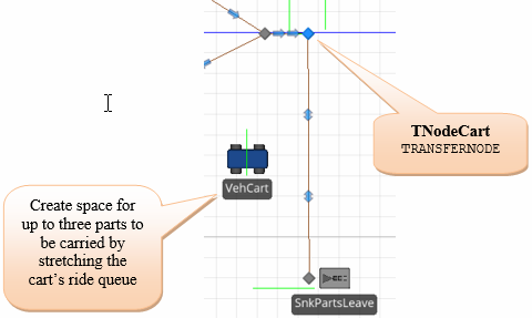
Figure 12.2: Adding a Vehicle
12.1.6 Change the TNodeCart TransferNode’s Ride On Transporter property to “Always,” meaning entities must always need a vehicle to move. The other option is “Conditional,” which allows you to specify a condition that must be true to require a transporter or the entity can move independently. Next, specify the “VehCart” as the Vehicle Name, which was just added (see Figure 12.3). Every time an entity passes through this node, it generates a ride request to be sent to the vehicle. The entity cannot continue until the vehicle is there to pick it up.
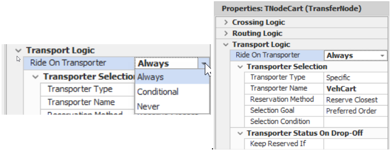
Figure 12.3: Setting up the Node to Have Entities Utilize a Vehicle
12.1.7 Use Figure 12.4 as a guide to set the VehCart’s Initial Desired Speed to four feet per second and Ride Capacity to three. Also, set the Initial Node(Home) to the TNodeCart node, which was just added, as this will be our vehicle’s home node. Leave the Routing Type specified as “On Demand,” meaning it will respond to requests for transportation from the stations as needed. Now, change the VehCart’s Idle Action property to”Park At Home” so that the vehicle will always go to the home node if there are no entities with ride requests.148 Otherwise, the vehicle will remain at the Sink until a ride request is generated.
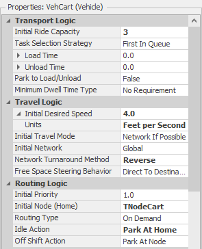
Figure 12.4: Vehicle Properties
| Process Type | Description |
|---|---|
| Initial Node (Home) | The node where the vehicle will start at the beginning of the simulation. |
| Routing Type | There are two different routing behaviors. The default “On Demand” option allows the transporter to act like a taxi and only move to pick up when an entity requests a ride. This mode will also enable the transporter to be used as a moveable resource that is seized and released. The “Fixed Route” type requires a sequence table for the transporter to transverse, like a bus route, to pick up entities on the route. |
| Idle Action | This property specifies what the transporter will do when it becomes idle (i.e., no transport or seize requests) when using the “On Demand” routing type. Go to Home and Park at Home. Send the vehicle to the home node, and one will force the vehicle to park in the station rather than visit the node. Remain In Place and Park at Node will do the same thing as the previous two but at the current node. The Roam action will have the transporter roam randomly through the simulation networking while waiting for an on-demand request. |
| Off Shift Action | It specifies what will happen when the transporter goes off shift and has the same options as the Idle Action except for the no “Roam” method. |
12.1.8 Run the simulation now to see how the cart works in the animation. As you can see, the VehCart is initially parked at the TNodeCart node Figure 12.5. By default, the parking animation queue is above the node149 and oriented from left to right. If there were more than one vehicle, they would be stacked on top of one another again, facing left to right in the facility, as seen in the right picture in Figure 12.5, where three carts are in the system.150
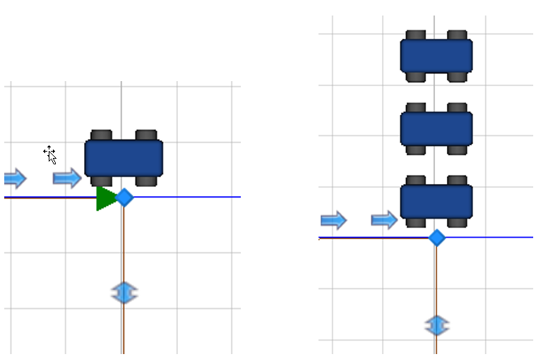
Figure 12.5: Vehicle is parked at the Home Node using Default Parking Station
12.1.9 To fix the issue of a single part riding out to one side, select the Ride Station queue on the Vehicle and change the Alignment from “None” to “Point” under the Appearance tab. Add an additional vertex to the queue to accommodate three parts and move the first orientation point from the bottom to the middle, as seen in Figure 12.6.
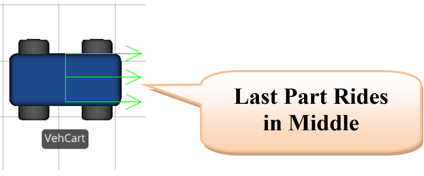
Figure 12.6: Changing the Orientation of the Riding Queue
12.1.11 By default, a parking location for a node is automatically added above the node, as seen in Figure 12.7. However, you should generally not utilize the default one since the location and/or shape of the parting station cannot be adjusted, and the orientation of the vehicles cannot be adjusted. Select the TNodeCart node by clicking it and then toggle the Parking Queue option in the Appearance tab to make it clearer. Next, a parking location is needed for the vehicle, or the vehicle will vanish when parked.151 Click on the TNodeCartnode and select “Draw Queue” from the Attached Animation Tab. Click on the ParkingStation.Contents. A cross cursor will now appear in the facility window. Left-click where you want the front of the queue to be and then right-click where you want it to end (before you right-click to end the queue, you could also continue left-clicking to add more vertices). Place it above the node so the vehicle will face downward, as seen in Figure 12.7. Click on the queue and the properties window to ensure the Queue State is ParkingStation.Contents. This queue will animate the parking station of the TNodeCart TransferNode for vehicles parked at the node. It can be oriented and placed at any location. Figure 12.7 shows the same scenario as Figure 12.5, but this time, we can orient the vehicles to point in the same direction as the path.
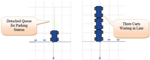
Figure 12.7: Vehicle is parked at the Home Node using the New Station
12.1.12 Run the simulation now to see how the cart works in the animation.
The model does not show how many parts are waiting for the cart at the transfer node, so it may be helpful to see how many are there at any given time in the simulation. To accomplish this, we can add an animated “Detached Queue” for the TNodeCart.
12.1.13 Click on the TNodeCart node and select “Draw Queue” from the “Appearance” Tab. Click on the “RidePickupQueue.”152 A cursor will now appear in the facility window. Left-click where you want the front of the queue to be and then right-click where you want it to end (before you right-click to end the queue, you could also continue left-clicking to add more vertices). As seen in Figure 12.8, arrange this detached queue in an “L” shape. Otherwise, an entity trying to enter the transfer node will be visible, and overlaying the “L” will show all the entities waiting for transportation.153
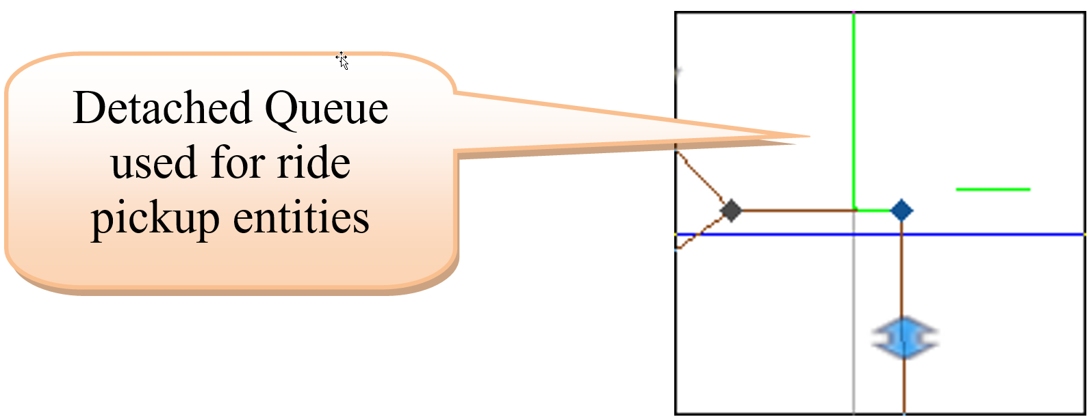
Figure 12.8: Ride Pickup Queue
12.2 Cart Transfer among Stations
Suppose that the transportation of parts among the stations, including entry and exit, is handled by two similar vehicles. These vehicles are different from the VehCart, which carries the parts to the warehouse sink. These carts will wait at the beginning of the circular network until they are needed.
12.2.1 Convert the one BasicNode that connects the four sources into a TransferNode by right-clicking and selecting the Convert to Type menu item. This will be necessary for parts entering the network from the sources to request transportation on the inside carts. Next, name this new TransferNode TNodeStart.
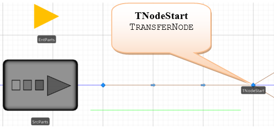
Figure 12.9: Changing the Start Node to a TransferNode
12.2.2 Now, add the inside carts by inserting another vehicle from the [Standard Library] into the model and naming it VehInsideCart. Shrink the vehicle leaving the ride station queue in the same position.
12.2.3 Make the VehInsideCart have an initial population of two154, allowing you to see the simultaneous behavior of multiple vehicles on the same path. The new vehicle will have the characteristics shown in Figure 12.10 (i.e., the Initial Node should be TNodeStart and the Idle Action property should be set to “Park at Home”). Select the “Transporting State” from the “Additional Symbols” and color it orange.
Notice that the Vehicle object is similar to the Entity object in that multiple instances, which we call “run-time” instances, can be created from the “design-time” instance of the VehInsideCart.155 “Design-time” occurs while you are putting instances of the objects onto the modeling. All the objects in the Facility window are initialized just before the simulation begins to execute. “Run-time” occurs when the simulation executes.

Figure 12.10: Properties of the InsideCart
12.2.4 We must ensure the inside carts can drop off parts and then return to the circular path. Since they obviously cannot go through the servers156, the inside carts would move to the input node of a server, drop off the part, and then go through free space to either the start node or to a pickup point rather than being on the network as discussed in Table 12.2. The easiest solution is to allow the carts to maneuver around the stations (i.e., add a Connector from the input to the output nodes of each station, as shown in Figure 12.11, making sure the direction of the link is correct.157
| Initial Travel Mode | Description |
|---|---|
| Network if Possible (Default Method) | The transporter will traverse the network from A to B if there is a path between those nodes. Otherwise, it will go via free space (i.e., a straight line). |
| Free Space Only | The transporter will only use free space. |
| Network Only | The transporter will only use the network and could be deadlocked if there is no path from nodes A to B. |
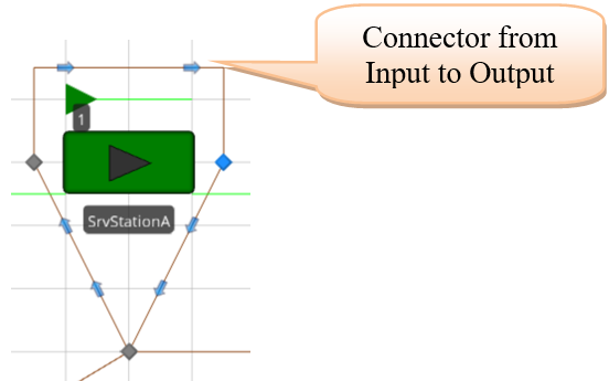
Figure 12.11: Ride Pickup Queue
12.2.5 Next, select the TNodeStart and the three output nodes (i.e., TransferNodes) of the station servers and specify the entities leaving these nodes to ride on a VehInsideCart, as seen in Figure 12.12.
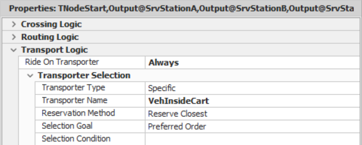
Figure 12.12: Use the Inside Cart
12.2.6 Finally, change the path between the exit node on the inside loop and the TNodeCart node to two one-way paths (i.e., add an additional path from the TNodeCart back to the basic node, making sure to make the path ten yards long). Also, change the path between the TNodeCart and the SnkPartsLeave to two one-way paths. Now, your overall model should look like the one in Figure 12.13.158
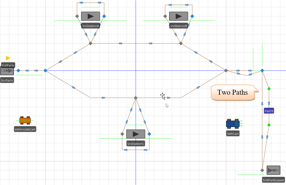
Figure 12.13: Model with Vehicles
12.2.7 Also, change the VehCart Population property Initial Number in the System to “2” so two carts will be available for outside transportation. The TNodeCart node should also be specified, as shown in Figure 12.14.
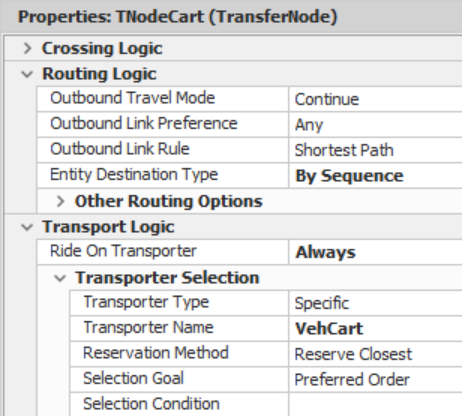
Figure 12.14: pecifying TNodeCart
12.2.9 The difficulty was the parts were not unloaded from the inside cart to be transported by one of the two outside carts to the Sink. The issue is that once the part has finished its last processing at a station, the next node in the sequence is the exit. Therefore, the inside cart takes part to its next destination (i.e., Input@SnkPartsLeave). To force the inside cart to drop off the parts at the TNodeCart node rather than transporting them all way to the exit, this node should be inserted into the four-part sequences right before the Input@SnkPartsLeave row for each part type, as seen in Figure 12.15.159
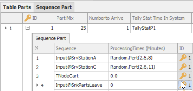
Figure 12.15: Ride Pickup Queue
12.2.10 Once all four sequences have been modified, save and execute the model. Observe the interacting behavior of the carts and notice how the carts park.
12.2.10.1 How do parts get transported from the inside workstations to the outside cart for transfer to the sink when the parts leave?
_______________________________________________
12.2.10.2 Is the queue ride parking for the TransferCart node needed anymore?
_______________________________________________
12.2.11 A few anomalies occur within the model. Notice how the inside carts will wait while they drop off a part when an outside cart is unavailable. When the part starts the drop-off process, the part entity visits the node, informing the part that it requires a vehicle to continue and, therefore, never completes the drop-off process to release the inside cart as shown in To fix this anomaly and other animation issues, delete the TNodeCart node and insert a new server named SrvPickup with an infinite capacity and zero for the processing time, as seen in Figure 12.17.
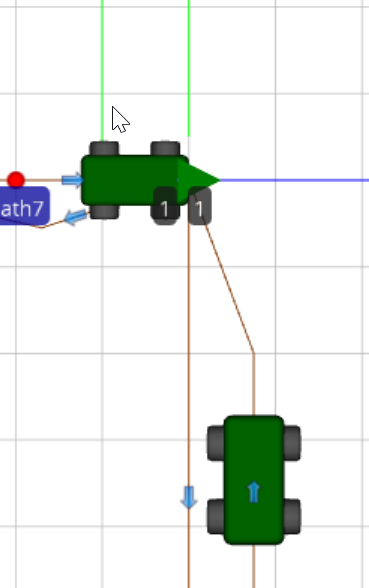
Figure 12.16: Inside Cart Stuck waiting for Entity to receive a Ride
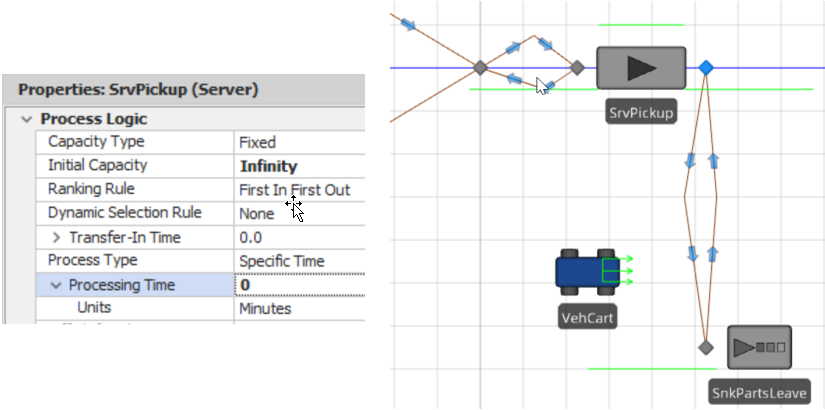
Figure 12.17: Adding a new Server as Pickup Point
12.2.12 Reconnect the two 10-yard paths from the path network to the input of the SrvPickup and the two 300-yard paths from the output node to the Sink.
12.2.13 For the sequence table, change the TransferCart node to the Input@SrvPickup and make the home node for the Cart the Output@SrvPickup node, as seen in Figure 12.18.

Figure 12.18: Changing the Sequence Table and Cart Home Node
12.2.14 Finally, request transportation on the Output@SrvPickup transfer node using the same information from Figure 12.14.
12.3 Other Vehicle Travel Behaviors (Fixed Route and Free Space Travel)
Let’s experiment with different vehicle specifications to create different cart behaviors. We will now explore both fixed-route travel (i.e., bus) and free space.
Fixed Route Travel
Currently, the inside cart travels wherever transport is needed among the stations, including entry and pickup based on the “On Demand” Routing Type specified in the vehicle definition. Suppose we want the cart to travel in a fixed sequence around all the service points in the model.
12.3.1 Insert a new Sequence Table from the Data tab for the vehicle Route Sequence named SeqInsideCart, as shown in Figure 12.19. Note that the sequence includes both the stations’ input and output nodes.

Figure 12.19: New Route Sequence for InsideCart
12.3.2 Select the VehInsideCart and set the Routing Type property to “Fixed Route” and the Route Sequence to the SeqInsideCart sequence table, as seen in the right picture of Figure 12.19.
12.3.3 Run the model and observe both the behavior of the cart(s) and the statistics on the cart’s performance.
12.3.3.1 Are both inside carts behaving as expected? What is their utilization?
_______________________________________________
12.3.3.2 Can you see the second cart? Why is its utilization 100%?
_______________________________________________
Because both carts are always active, their utilization is 100%, and the two carts ride (i.e., overlap one another) in the same location. So if we are to see carts, we need to interrupt the constant motion or have the two carts start at different times (i.e., have a Source create them at different times so there is space between them). There are several ways to achieve the result.
12.3.4 Change the Load Time of the VehInsideCart to an Exponential(0.5) minutes, which will cause the vehicle to pause while loading each part. Save and run the model, observing the cart’s behavior.160
12.3.4.1 What happens to both inside carts?
_______________________________________________
Free Space Travel
Rather than travel on a specific path between stations, vehicles, workers, and entities can travel in “free space.” SIMIO needs the “location” of the various nodes to do this. In other words, it will assume that your model is “to scale,” as it might be if the animation layout is based on computer-aided drawing (CAD) software. It’s essential to recognize that the time it takes for parts to be moved by vehicles depends on the distance the vehicle travels and its travel speed161. To illustrate the free space travel, let’s treat our animation as though it came from a CAD drawing.
12.3.5 Save the current model as Chap12.3Step12.3.6 and eliminate all the paths and nodes between the stations and the SrvPickup so that travel is unrestricted, as seen in Figure 12.20.
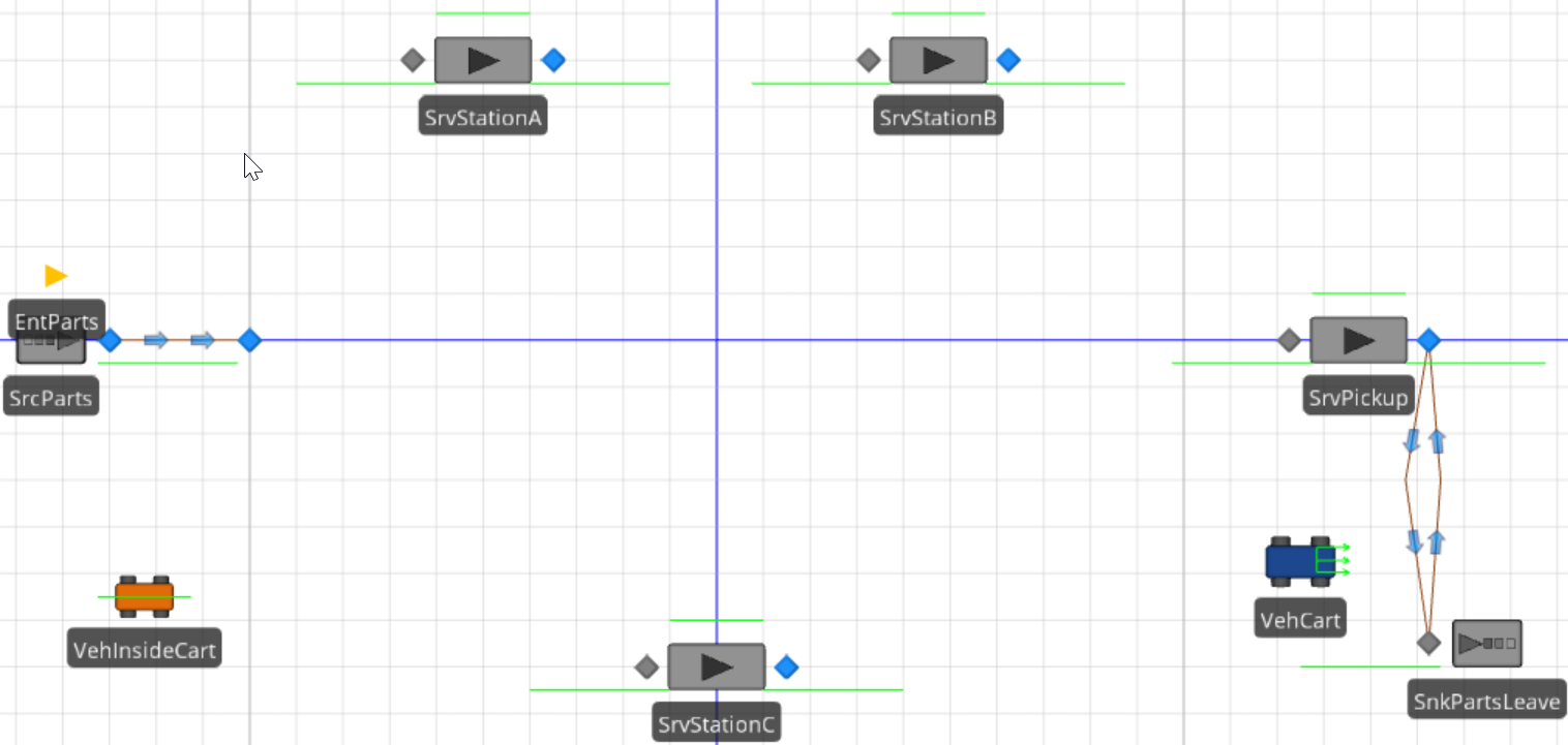
Figure 12.20: Layout to Scale: No Paths
12.3.6 Modify the VehInsideCart “Travel Logic” and “Routing Logic” as Figure 12.21. In this case, we could change Initial Travel Mode to “Free Space Only” or leave it at the default “Network if Possible,” showing there is no travel network – meaning the vehicle must use free space. We are also routing “On Demand,” and the Idle Action is set to “Remain Place.”
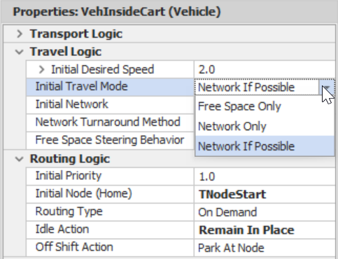
Figure 12.21: Travel Logic and Routing Logic
12.3.8 The part entity automatically floats through free space from the output node of the SrcParts to the first node in the sequence because the output node of the Source says use by sequence to determine the part’s next destination. Since the default travel mode is “Network if Possible” and there are no direct paths from the Source to the nodes, the part moves in free space. This travel will bypass the TStartNode, which specifies the entity’s need to ride on a transporter. Table 12.3 outlines two ways to fix the issue.
| Object | Property | Description |
|---|---|---|
| Output@SrcParts | Ride on Transporter | Change the output node’s “Ride on Transporter” property to “Always,” specifying the VehInsideCart as the transporter. |
| EntParts | Initial Travel Mode | Change the Initial Travel Mode of the entity to “Network Only,” forcing it to use the connector to the TStartNode. |
12.4 Conveyors: A Transfer Line
SIMIO provides for two kinds of conveyor modeling concepts: accumulating and non-accumulating. An accumulating conveyor allows parts to queue at its end, but the conveyor keeps moving. This approach might model a belt conveyor whose parts rest on “slip sheets” that allow the belt to continue to move. A non-accumulating conveyor must stop until the on-off operation is completed. This concept might apply to an overhead conveyor with parts on carriers. SIMIO conveyors do not have on/off stations, so a transfer line must be modeled as a series of individual conveyors. Since the transfer line stops, the non-accumulating concept applies. However, the individual conveyors will need to be synchronized.
Suppose a continuous conveyor transfer line handles the transfer among stations in the manufacturing cell, possibly in a loop with on/off stations. When a part is at an on/off station, the entire line pauses until the part has been placed on or taken off the conveyor. It takes between 0.5 and 1.5 minutes to load/unload the parts from the nodes.
12.4.1 Reopen the last model from Chapter 5 and save it with a new name. Now, change the arrival rate of the Source to Random.Exponential(15).
12.4.3 Also, the symbols for the parts should be modified so they are one meter wide by one meter in length and one-half meter in height. Select the EntParts ModelEntity, and change the size under the General→Physical Characteristics→Size properties for the first active symbol. After selecting a different active symbol, you must deselect and reselect it to see its size. We will need to be a little more specific about these sizes as we size the conveyors. We created these symbols from the “Project Home” tab in the “Create” section, clicking on “New Symbol” and selecting “Create a New Symbol.” when creating the symbol, we paid close attention to its size (the grid is in meters).
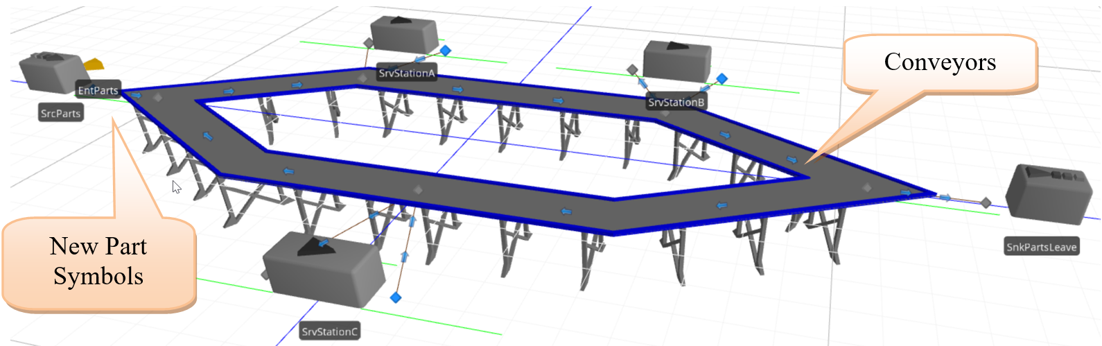
Figure 12.22: 3D View with Conveyors
12.4.4 Next, the properties of the conveyors need to be specified. It is convenient to use the “Spreadsheet View” by right-clicking on one of the conveyors and selecting Open Properties Spreadsheet. The lengths from the previous paths (recall they were 25, 35, 20, 30, and 40 yards) do not need to be modified. All five conveyors should have a conveyor speed of 0.5 meters/second for each conveyor. Set each conveyor’s Accumulating property to False (i.e., the selection boxes should be unchecked).
12.4.5 Choose the Cell Location option in the Entity Alignment property. Selecting this option causes the conveyor to be conceptually divided into cells. Parts going onto the conveyor will need to be placed into a cell. Therefore, choose the number of cells equal to the number associated with the conveyor length. Otherwise, if you select Any Location for the Entity Alignment, a part can go onto the conveyor anywhere, even interfering with another part (i.e., think about the baggage conveyor at an airport).
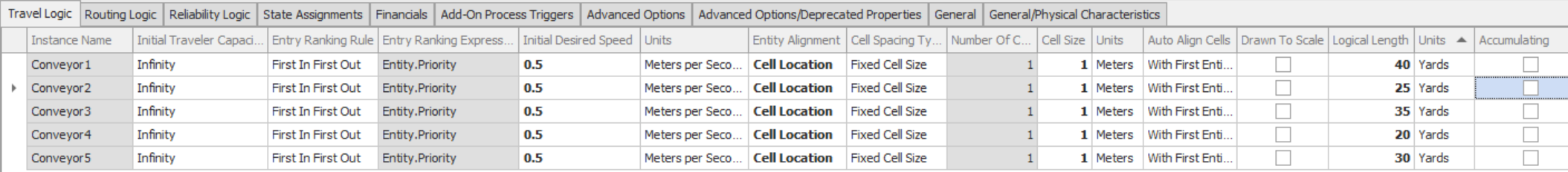
Figure 12.23: Specifying Properties for all Five Conveyors of the TransferLine (Spreadsheet View)
12.4.6 Since the transfer line consists of multiple conveyors rather than a continuous one, the conveyors have to be synchronized so that when parts enter an on/off location on the transfer line, the entire line, which is a set of conveyors, stops to await the on/off operation.163 First, define a new discrete state variable of type integer (from the Definitions tab) for the Model named GStaNumberNodesWorking. This variable will represent the number of on/off locations currently either putting parts onto or taking parts off the transfer line. When this state variable is zero, the transfer line is running, and when this variable is greater than one, the transfer line should be stopped.
12.4.7 Let’s now insert a new “process.” From the “Processes” tab, select “Create Process” and name the new process On_Off_Entered. The process will consist of the steps shown in Figure 12.24.

Figure 12.24: Process when Entering/Leaving the Transfer Line
- When a part reaches an on/off operation, the Assign step needs to increment the GStaNumberNodesWorking by one, and all conveyors need to be stopped by setting their desired speed to zero (see Figure 12.25).164
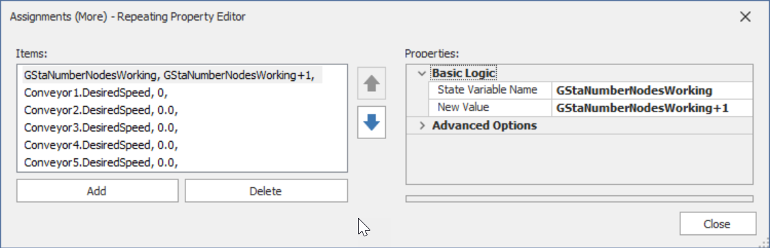
Figure 12.25: Incrementing the Number of Nodes Working and Shutting the Conveyors
- The Delay step will be used to model the on/off time, which is assumed to be uniformly distributed with a minimum of 0.5 and a maximum of 1.5 minutes.
- The second Assign step will now decrement the GStaNumberNodesWorking by one.
- The Decide step is based on the condition that GStaNumberNodesWorking==0, meaning no other on/off stations are busy loading/unloading the transfer line.
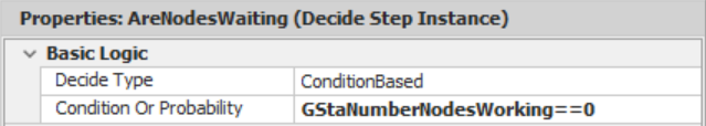
Figure 12.26: Decide Step Option
- The last Assign step will turn the conveyors back on. SIMIO stores all times internally in meters per hour. If the state variable has units, these can be specified in the assignment. Make sure you change the units to meters per second, or an assignment of 0.5 would be treated as 0.5 meters per hour.165 You can convert the original specification of 0.5 meters per second to 1800 meters per hour to be consistent with how SIMIO will interpret the assignment and avoid having a conversion each time. Figure 12.27 shows the conveyors being turned back on.
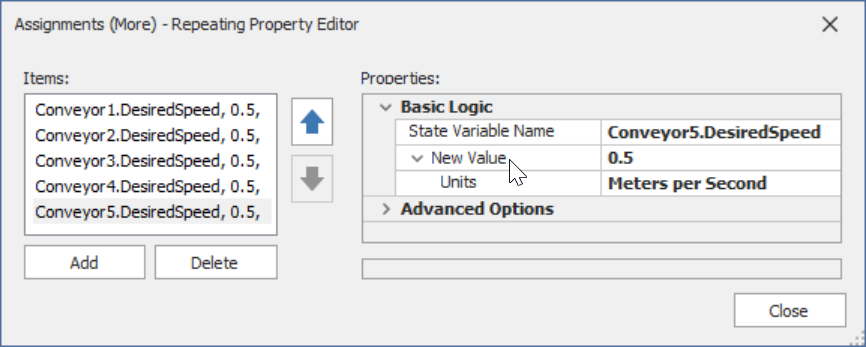
Figure 12.27: Turning the Conveyors Back On
12.4.8 Finally, the On_Off_Entered generic process must be invoked appropriately (i.e., every time a part is loaded or unloaded to the transfer line). Select the On_Off_Entered as the add-on process trigger for all the nodes and one path (i.e., the path to the exit SnkPartsLeave) as specified in Table 12.4.
| Add-On Process Trigger | Which Object the Trigger is Associated |
|---|---|
| Exited | Output@SrcParts (TransferNode) |
| Entered | Input@StationA (BasicNode) |
| Exited | Output@StationA (TransferNode) |
| Entered | Input@StationB (BasicNode) |
| Exited | Output@StationB (TransferNode) |
| Entered | Input@SnkPartsLeave (BasicNode) |
| Entered | Input@StationC (BasicNode) |
| Exited | Output@StationC (TransferNode) |
Triggers that Need to Go Through the On/Off Process Logic
12.4.9 Run the simulation for 40 hours at a slow speed to ensure each part follows its sequence appropriately and answer the following questions.
12.4.9.1 How long are all part types in the system (enter to leave)?
_______________________________________________
12.4.9.2 What is the utilization of each of the Servers?
_______________________________________________
12.5 Machine Failures in the Cell
Failures are a part of most mechanical and other systems. SIMIO provides methods to model these failures within the “Reliability Logic” section of the Server (and other objects), as seen in Table 12.5. In the case of the transfer line, we also need to shut it down while a machine is being repaired.166 Let’s assume that SrvStationC is an unreliable machine. In particular, we will assume that the MTBF (Mean Time Between Failures) is exponentially distributed with a mean of ten hours, while the MTTR (Mean Time To Repair) is modeled with a Triangular distribution (0.5, 1, 2) hours.
| Failure Type | Description |
|---|---|
| No Failures | Specify there will not be a failure. |
| Calendar Time Based | Specify the calendar time that needs to transpire before a failure will occur. |
| Event Count Based | Specify the number of times a particular event occurs that will cause the server to fail. |
| Processing Count Based | Specify the number of entities that are processed before a failure (e.g., after 100 entities, we need to change the tool). |
| Processing Time Based | Specify the total processing time that the server works before a failure (e.g., after 100 hours of work, we need to change the oil in the machine). |
12.5.1 In the “Reliability Logic” section for the Station C Server, specify the Failure Type to be “Calendar Time Based” and the Uptime Behavior to be Random.Exponential(10) with units of hours, and the Time To Repair should be Random.Triangular(0.5,1,2) with units of hours as seen in Figure 12.28. Remember that the server is failing, which means that all the capacity associated with this server fails (the capacity for this server is scheduled, but it changes between 1 and 2).
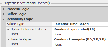
Figure 12.28: Turning the Conveyors Back On
12.5.2 When the SrvStationC fails, the entire transfer line should be shut down and then started back up once the station has been repaired. Select SrvStationC and create new Add-On Process Triggers, “Failed” and “Repaired,” to produce new processes SrvStationC_Failed and SrvStationC_Repaired. The “Failed” been repaired. In SrvStationC_Failed, use an Assign step to turn off all of the conveyors by setting their DesiredSpeed to zero. In the SrvStationC_Repaired, use an Assign step to turn back on the conveyors if there are currently no nodes loading/unloading (i.e., setting the DesiredSpeed = 0.5 meters per second for all conveyors) as seen in Figure 12.29.167
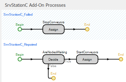
Figure 12.29: Failed and Repairing Process Triggers
12.5.3 Also, the On_Off_Entered process should not start up the transfer line if the SrvStationC has failed and is currently On_Off_Entered process so the conditional expression becomes the following.168
(GStaNumberNodesWorking==0) && (SrvStationC.Failure.Active==False)169
12.6 Sorting Conveyors
Now, we find out that the output from the conveyor system is another system of conveyors that sorts the parts into destinations. The parts that exit the manufacturing cell are routed to an accumulating conveyor at a labeling machine. From the labeling machine, the parts are conveyed to one of four sinks corresponding to the specific part type, as seen in Figure 12.30. The four conveyors directly in front of the sinks are accumulating conveyors. These conveyors keep moving, and parts are allowed to queue, although the sinks pose no barrier to exit in this case. The rest of the conveyors are non-accumulating.
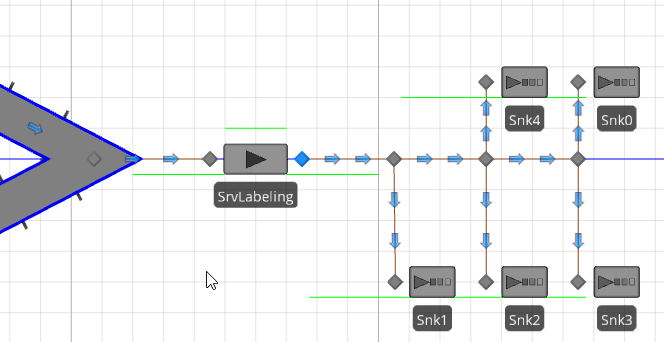
Figure 12.30: Labeling and Sorting Conveyors
12.6.1 Remove the original SnkPartsLeave and replace it with a SrvLabeling. The labeling processing time follows a Triangular(1,2,3) minutes and has a capacity of “1.” Since the labeler will be supplied by an accumulating conveyor from the inside set of conveyors (i.e., the BasicNode), set the Input Buffer capacity property to zero because it is not needed and there is no delay in off-loading to this conveyor.
12.6.2 Add three BasicNodes to follow the SrvLabeling and name them BNode1, BNode2, and BNode3 in that order. These are conveyor diverters that will send the sorted parts to their destinations. Add three sinks, Snk1, Snk2, Snk3, and Snk0, to represent the destinations for parts of type 1, 2, 3, and 0, respectively. Connect the objects with conveyors according to Table 12.6.
| From/To | Conveyor Type | Conveyor Length | Conveyor Speed |
|---|---|---|---|
| BasicNode to SrvLabeling | Accumulating | 10 meters | 1.0 meters per second |
| SrvLabeling to Basic1 | Non-Accumulating | 10 meters | 0.5 meters per second |
| BNode1to Snk1 | Accumulating | 10 meters | 0.1 meters per second |
| BNode1to BNode2 | Non-Accumulating | 10 meters | 0.5 meters per second |
| BNode2 to Snk2 | Accumulating | 10 meters | 0.1 meters per second |
| BNode2 to Snk4 | Accumulating | 10 meters | 0.1 meters per second |
| BNode2to BNode3 | Non-Accumulating | 10 meters | 0.5 meters per second |
| BNode3to Snk3 | Accumulating | 10 meters | 0.1 meters per second |
| BNode3to Snk0 | Accumulating | 10 meters | 0.1 meters per second |
12.6.3 For the part’s sequence table, replace the Input@SnkPartsLeave entries with Input@SrvLabeling. Next, add the sink node destinations associated with the part types. Figure 12.31 shows part of the table, and you can insert the last placement at the end to maintain the sequence.
Figure 12.31: Changes to Sequence Table
Next, change the Output@SrvLabeling node Entity Destination Type to By Sequence. There is no need to add intermediate nodes (the BasicNodes) since SIMIO can find the designations from the SrvLabeling.
12.6.4 Select all the conveyors and add the conveyor path decorators, as seen in Figure 12.32.
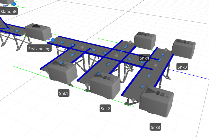
Figure 12.32: Conveyor with Path Decorators
12.6.6 Run the simulation for 40 hours.
12.6.6.1 What is the average number of parts accumulating on the conveyor before the labeler?
_______________________________________________
12.6.6.3 Why does the OutputBuffer of the labeler have content?
_______________________________________________
12.7 Commentary
- Material handling can be a substantial cost of production and thus is of great interest to many companies. Vehicles and conveyors provide considerable flexibility in modeling material handling.
- The modeling of cranes has not been included in this chapter. These are a complex category of materials handling. However, SIMIO has developed a special library for cranes that can represent a wide variety of overhead and floor cranes. In particular, there is a 3D animation of the cranes to reflect that cranes operate in three dimensions. This package is highly recommended.
The Network Turnaround Method can be changed for example to “Reverse” so the cart would go forward to the exit and then look as if it backs up to the TNodeCart node. By default it will turn around and move forward back to the home TNodeCart node.↩︎
Note the familiar green line that represents the animated queue line is not visible in this case.↩︎
Unlike entities, the default number of vehicles is one and can be changed in the Population properties. Also, a Source can create vehicles.↩︎
The parking queue is again just for the animation since the vehicle is physically at the node even though it cannot be seen.↩︎
If added just generic animated queue now, change the Queue State property to TNodeCart.RidePickupQueue where TNodeCart is the name of the transfer node where the parts are being picked up. Your transfer node’s name may be different.↩︎
These queues are for animation purposes only. The parts physically reside at the entrance of the node and one will always be visible as the others will stack up underneath. In later chapters, the notion of a Station to hold entities will be discussed.↩︎
The fact that the property description says “Initial number in System” should indicate that vehicles can be added and removed from the simulation during the simulation execution (something that is left to a later chapter).↩︎
We will see that the Worker object can also have run-time instances.↩︎
By default, Workers and Vehicles will not enter fixed objects like Servers, Sinks, Combiners, etc. One solution is to create a connector that leaves the input node to the transfer node, and another from the transfer node to the output node to allow pickup.↩︎
Recall that connectors take up zero time and have zero length in the model. Basically, the server's inputs and outputs are really the transfer nodes of the circular path.↩︎
One can use bidirectional paths but this can lead to bottlenecks and deadlock as vehicles, workers, and entities can only be going in one direction and must wait for all items to clear path before the direction can be reversed. It is always better to use two separate paths.↩︎
The easiest way to insert the node into the sequence is to select the Input@SnkPartsLeave row and then click the Insert Row button in the Data section of the Table tab. Also, doing it part by part by accessing the related table from the Table Parts is easier.↩︎
We could have also added an unload time to simulate the time taken to unload parts at the various stations.↩︎
When vehicles move entities, it’s the speed of the vehicle that determines how fast it traverses a distance and not the entity speed.↩︎
Note you can use the Ctrl key to select all five paths and convert them all at once.↩︎
The synchronization is not exact since the occupied cell of the upstream conveyor is not known to the downstream conveyor and parts from a cell may conflict with parts arriving from the upstream conveyor (i.e., SrcParts).↩︎
You will need to select the Assignments (More) button in the Assign step.↩︎
The presumption of a standard internal time probably represents a choice of efficiency over ease of use, since determining the original time units would represent some additional computational effort.↩︎
The tremendous cost of downtime due to everything on the line becoming idle is one of the reasons why transfer lines and similar highly automated processes are becoming relatively rare.↩︎
Copy the Decide and Assign steps from the On_Off_Entered process and remove the increment of the GStaNumberNodesWorking.↩︎
Object.Failure.Active function will return true if the current object has failed.↩︎
Notice that SIMIO utilizes C# logical operators (i.e., == for equality, && for “And” statement, and || for the “Or” statement).↩︎