Simulation Modeling with Simio - 6th Edition
Chapter
6
Assembly and Packaging: Memory Chip Boards
A standard simulation environment in production is assembly and packaging. What makes these operations challenging is that entities are being combined together. The way they are combined can be complicated. Sometimes, the assembly is temporary, and the assembly (called a batch) must be separated later. These considerations cause us to have an interest in the Combiner and Separator object.
6.1 Memory Board Assembly and Packing
Memory boards have memory chips inserted into them at an assembly operation, whose capacity is four. Each memory board requires four chips. Memory boards and individual memory chips arrive randomly, so the assembler waits for four chips of the same type and one board to be available before doing the assembly. After the board is assembled, it is sent to one of three packing stations, each of which has one worker. Boards are sent to the packing station with the smallest queue. Figure 6.1 depicts the memory board assembly and packing process.
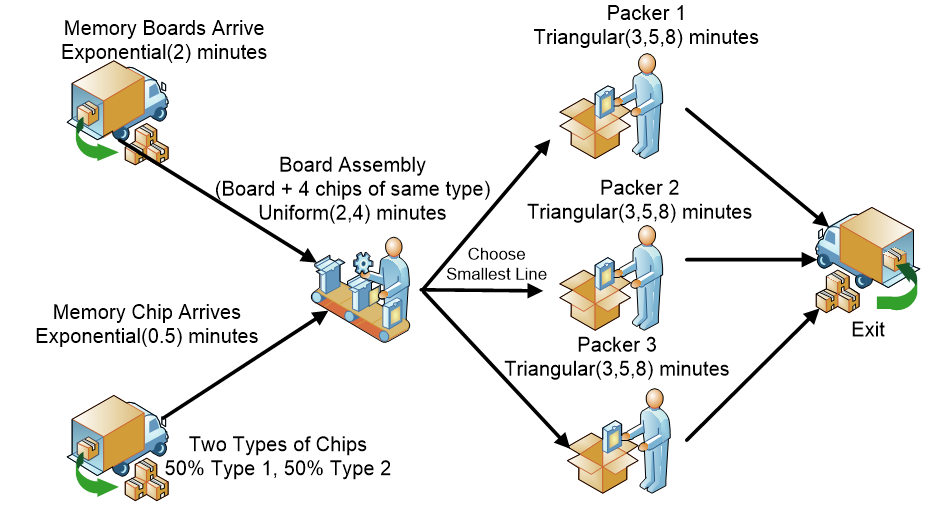
Figure 6.1: Memory Board Assembly and Packing
The basic numerical characteristics of the assembly problem are found in Tables 6.1 and 6.2.
| From | To | Travel Time (minutes) |
|---|---|---|
| Memory Board arrivals | Board Assembly | 4 minutes |
| Memory Chip arrivals | Board Assembly | 5 minutes |
| Board Assembly | Packer Station 1 | Pert(10,12,15) minutes |
| Board Assembly | Packer Station 2 | Pert(5,7,10) minutes |
| Board Assembly | Packer Station 3 | Pert(4,5,7) minutes |
| Any Packer Station | Exit | 3.5 minutes |
| Memory Board Model Inputs | Distribution |
|---|---|
| Interarrival time for Memory Boards | Exponential(2) minutes |
| Interarrival time for Memory Chips | Exponential(.5) minutes |
| 50% of Memory Chips are of type 1, and 50% are of type 2 | Discrete |
| Board Assembly processing time | Uniform(2,4) minutes |
| Packing time for all Packers | Triangular(3,5,8) minutes |
6.1.1 Create a new model that has two Sources named SrcMemoryBoard and SrcMemoryChip (i.e., one for boards and one for memory chips). Add two ModelEntities into the model, one for boards named EntMemoryBoard and one for memory chips named EntMemoryChip.58 Ensure the Entity Type property of the two sources will create the appropriate entity type.
6.1.2 Give the entity type associated with boards a different symbol, as seen in Figure 6.2. You can use one of the stock SIMIO symbols or download a symbol from the Trimble 3-D warehouse, as done in Chapter 2. You can also make your own symbols in the “Project Home” tab by clicking the “Create New Symbol” menu item from the New Symbol dropdown in the “Create” section. In the properties window, name the symbol SymMemoryBoard. When creating a new symbol, you should give the symbol “height” by specifying a value (in meters). In the case shown in Figure 6.2, a rectangle was created with a line width of 0.1 meters and a height of 0.25 meters59. The rectangle was given a fill color of grey with a line color of green. One should not worry about the exact specifications since the symbol can be adjusted manually.
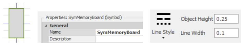
Figure 6.2: Symbol: Changing the Name and Specifying the Height and Line Width
6.1.4 For the memory chips, add an additional symbol60 since we have two different types of memory chips. You should color the second symbol a different color (e.g., red) to distinguish them in the system.61
6.1.5 Insert a Combiner named CmbBoardAssembly into the model for the assembly operation, as shown in Figure 6.3, which will batch/combine a parent entity object with a member entity object. Set the initial capacity of the CmbBoardAssembly to four and the processing time to Uniform(2,4) minutes. The combiner has two input nodes (i.e., a ParentInput and a MemberInput). The parent object is the board, while the member object is the memory chip. Connect the two sources via time paths to the appropriate nodes using the time specified in Table 6.1.
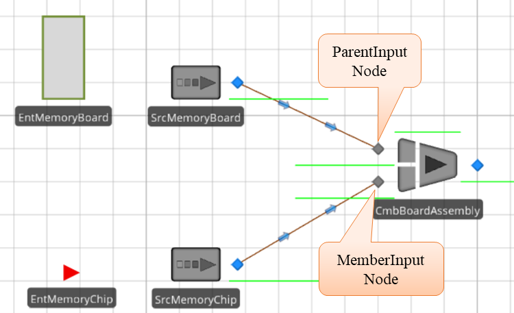
Figure 6.3: Initial Memory Board Model
6.1.7 To make the state variables clear when they are used in various places in a model, we prefix a ModelEntity state variable with ESta… and a Model global state variable with GSta….
6.1.8 Recall a board requires four identical memory chips. Therefore, the Combiner should batch four members of the same type. Let’s add an entity-based state variable to distinguish between the two types of memory. Select the ModelEntity in the [Navigation] panel and then choose the “States” section from the “Definitions” tab. Since there are two distinct chip types, insert a new “Integer State Variable” named EStaChipType, as seen in Figure 6.4.
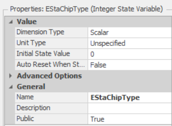
Figure 6.4: Specifying the ModelEntity Integer State Variable
6.1.9 Returning to the “Facility” tab of the Model, click on the SrcMemoryChip source. To assign the new EStaChipType variable, a State Assignment, Before Exiting, will be specified, which will make the assignment right before the entity leaves the source. Expand the State Assignment section. Then click on the box to the right of Before Exiting, which brings up the “Repeating Property Editor,” and add the following property.
Since it is equally likely the chip will be type one or type two, a random discrete distribution will be used to assign the EStaChipType value a one or a two (see Figure 6.5).
State Variable Name: ModelEntity.EStaChipType
New Value: Random.Discrete(1, 0.5, 2, 1.0)63
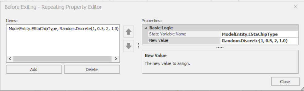
Figure 6.5: Setting the Entity’s Chip Type in a State Assignment
6.1.10 Since the chip entities can be distinguished, batch four members (i.e., chips) at the Combiner by specifying Match Members as the Matching Rule with ModelEntity.EStaChipType as the Member Match Expression property, as seen in Figure 6.6.64 Then, expand Other Batching Options and change the value of Must Batch Simultaneously to True. All four chips must be at the combiner before batching begins.
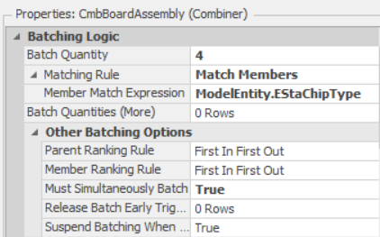
Figure 6.6: Specifying the Matching Logic in the Combiner
6.1.11 Insert three Servers (i.e., SrvPacker1, SrvPacker2, and SrvPacker3) one for each packer with the appropriate processing times (see Table 6.2) and one Sink named SnkExit (see Figure 6.7). Utilize TimePaths to connect the assembly to the packers and the packers to the exit. Specify the appropriate travel times specified in Table 6.1 for the time paths between the assembly and the packers, but do not specify the times between the packers and the exit quite yet.
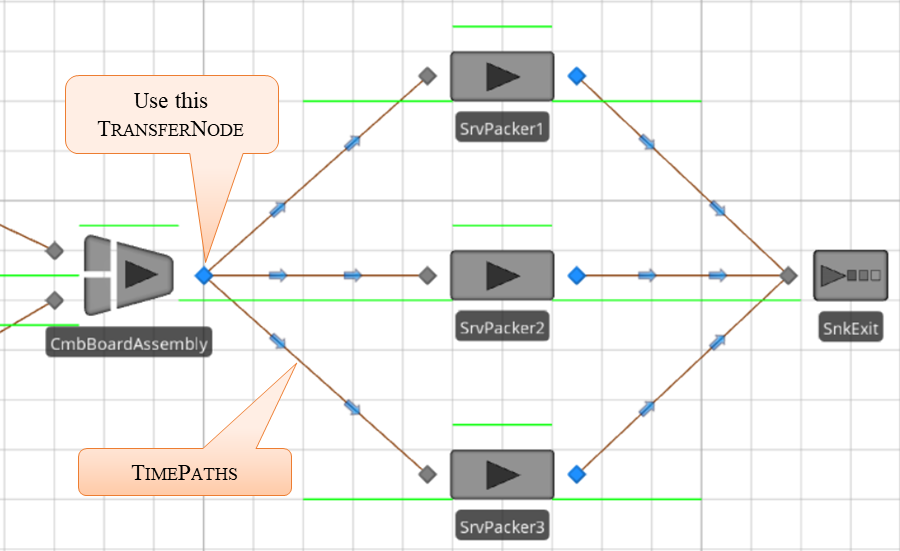
Figure 6.7: Packing Portion of the Model
6.1.12 Recall the board assemblies need to choose the packer with the smallest number assigned to it. At the output TransferNode associated with the Combiner, the branching decision needs to be specified using the Entity Destination Type property specification in the TransferNode.
6.1.13 Once the board finishes assembly in the combiner, it can select one of the three destinations: Input@SrvPacker1, Input@SrvPacker2, or Input@SrvPacker3, depending on the number of boards already assigned/designated to each packer. Create a new Node List (see Definitions→Lists tab) named LstPackers, beginning with Input@SrvPacker1, as seen in Figure 6.8. Lists are necessary whenever you need to choose from a set of objects (e.g., nodes, resources, etc.).
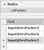
Figure 6.8: Node List for Selecting the Best Packer
6.1.14 Now, at the TransferNode, specify that entities should transfer to the destination according to the following properties, as seen in Table 6.3. Once you specify the Selection Goal property, you need to expand it to access the Selection Expression. We need an expression to evaluate the “shortest queue.” However, do we just mean the number in the respective queues? Probably not. How about including the number of entities being processed in the Servers and the number of entities traveling to the Server.
| Property | Value |
|---|---|
| Entity Destination Type: | Select from List |
| Node List Name: | LstPackers |
| Selection Goal: | Smallest Value |
| Selection Expression: | Candidate.Node.NumberTravelers.RoutingIn + Candidate.Server.InputBuffer.Contents.NumberWaiting + Candidate.Server.Processing.Contents.NumberWaiting |
| Selection Condition: | (Leave Blank65) |
The Candidate designation is a “wildcard” reference that takes on the identity of the object it references. Here, it refers to the node to which the entity is being routed and the particular InputBuffer and Processing queue of the Server at the end of the path. In this example, the word Candidate is replaced by each node in the list and the expression is evaluated. In a later chapter, AssociatedStations functions will be used to simplify this expression. Leave the Selection Condition blank and leave the Blocked Destination Rule as the default value.
6.1.15 Since the travel time to exit is the same for all packers and we don’t expect to change it during the simulation, let’s specify the travel from the packers to the exit using a “Model Property” via the “Definitions” tab. Insert an Expression property from the “Standard Property” dropdown named TimeToExit and give it a Default Value of 3.5 with Unit Type of Time with Default Units as Minutes. Since this is an “Expression” property, one could specify an expression for the time to exit (for example, Random.Uniform(2,10)), while a numeric property only allows constant (i.e., 3.5).
6.1.16 Now you can specify  as a referenced property for the Travel Time on each of the time paths to the exit66. Now, if you want to change the travel time on these three paths at the same time, only the new property has to be changed, or you want to experiment with the impact of this time. You can access the model properties by right-clicking on the Model in the [Navigation] and then expanding the “Controls” category to access our new property, as seen in Figure 6.9.67
6.1.17 The Model properties become controls for the simulation. These can be changed at the beginning of any run. Furthermore, they become changeable scenario properties in experiments, as we saw earlier in Chapter 2.
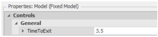
Figure 6.9: Changing the Properties of the Model
6.1.18 Save and run the model for 10 hours, answering the following questions.
6.1.18.1 How long do the entities stay in the system (enter to leave)?
_______________________________________________
6.2 Making the Animation Reveal More Information
Let’s first fix the memory board animation so the “chips” look attached to the board.
6.2.1 Select the EntMemoryBoard ModelEntity and insert the BatchMembers queue from the “Attached Animation” in the “Queue” dropdown. Position it on top of the EntMemoryBoard, as seen in Figure 6.10.
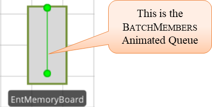
Figure 6.10: Added Batch Queue
To put an object on top of another, you need to select the object and hold down the Shift key to stack the queue on top of the memory board symbol. It’s probably best to do this while switching back and forth from 2-D to 3-D.68
6.2.2 Now, let’s use the color of the memory chip symbol to designate the two different chip types. To do this, click on the EntMemoryChip ModelEntity and click on “Add Additional Symbol” in the “Additional Symbols” section of the” Symbols” tab. You can color one symbol red and the other green by simply selecting one of the “Active Symbols” and changing its color. Please note that these two symbols are numbered zero and one (not one and two).
6.2.3 Next, we need to “assign” the colors to the different chip types. Select the SrcMemoryChip Source. Expand State Assignments and click on the box to the right of Before Exiting since we want to assign the color before the entity leaves the source. This brings up the “Repeating Property Editor.” Add an additional property with the following characteristics (see Figure 6.11).
State Variable Name: ModelEntity.Picture
New Value: ModelEntity.EStaChipType-169
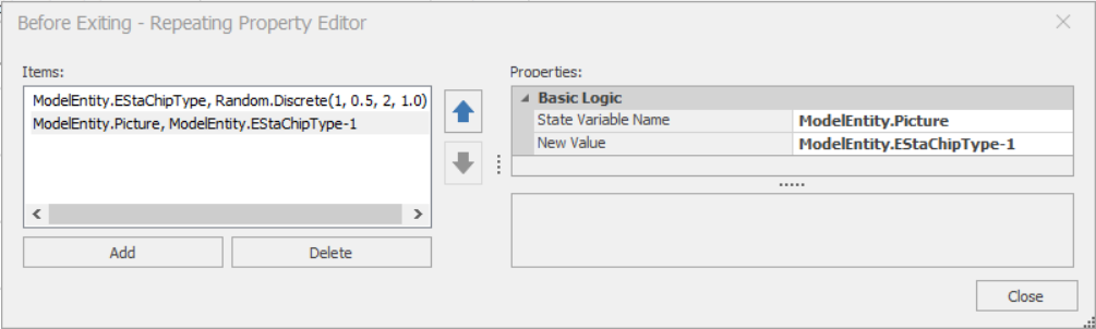
Figure 6.11: Changiing the Chip Entity to have a Different Color
Unlike a property, a “state variable” can be changed throughout the simulation. Here, the picture is a SIMIO-defined characteristic of the entity (in some simulation languages, it is called an attribute of the entity).
6.2.5 Suppose now we want the symbol leaving the packing station to represent a “package.” There are several ways one might do this. One easy way is to make a State Assignment by selecting Before Exiting at the Packing stations. Now, at one of the Packing stations, bring up the Repeating Property Editor and, this time, add:
State Variable Name: ModelEntity.Size.Height
New Value: 1
6.2.6 You may need to experiment with the value. The idea is to change the memory board’s “height” so that it encases the “chips” so they cannot be seen (i.e., hides the batch members inside the board).
6.2.7 Run the model and adjust the “height” so it shows a “package” leaving the packer. You will need to add this change in “height” at each packer station when the entity exits.
6.2.9 Save the model as Chapter 6.2.spfx and run the model for 10 hours.
6.2.9.1 How long are the entities in the system (enter to leave)?
_______________________________________________
6.2.9.2 What is the utilization of the CmbBoardAssembly?
_______________________________________________
6.2.9.3 What is the utilization of each of the packers?
_______________________________________________
6.2.9.4 What is the average number in the MemberInputBuffer?
_______________________________________________
6.3 Embellishment: Other Resource Needs
Sometimes, capacity is not just limited to objects like Servers and Combiners. The limitation may not even be fixed at a particular location. For example, suppose the board assembly requires a particular fixture to assemble the chips to the board. Furthermore, that fixture is used to transfer the assembly to packing. For each assembly, the fixture must be first obtained from the packing operation, which takes about three minutes, and we will relax the assumption. Let’s assume there are ten identical fixtures available for assembly-packing, and once they are released at the pacing, they can be used immediately at the assembly.
6.3.1 First, drag and drop a Resource object70 onto the modeling canvas, maybe just below the Combiner, as shown in Figure 6.12. Name the resource ResFixture and specify an Initial Capacity of 10 (we won’t be changing its capacity in this case).71
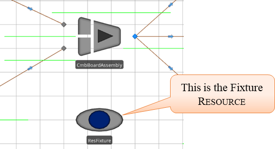
Figure 6.12: Adding a Fixture Resource
Next, logic needs to be specified on how this Resource is to be utilized. The fixture will be “seized” just before the assembly operation begins and then released just after the packing operation finishes.
6.3.2 For the CmbBoardAssembly Combiner, select the Secondary Resources, the Other Resource Seizes, and the Before Processing, as seen in Figure 6.13. Click the ellipses box to bring up the Repeating Property Editor for seizing resources and request one unit of the ResFixture resource capacity to be seized. We won’t worry about which fixture is seized since they are identical.
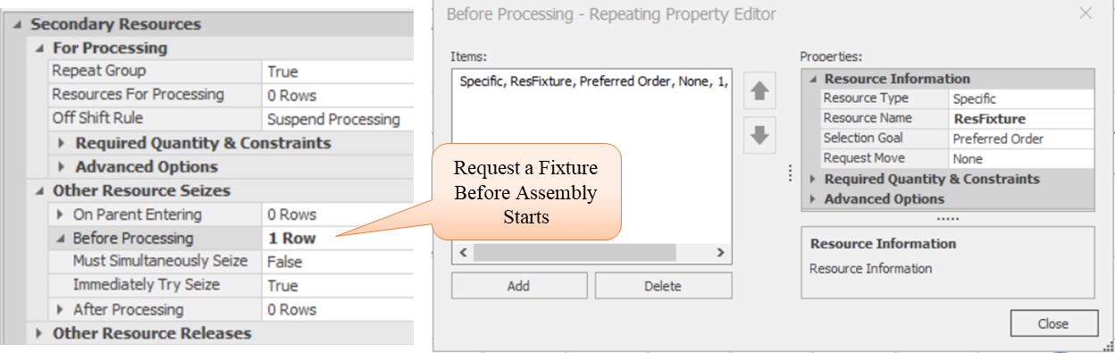
Figure 6.13: Seizing One Unit of the Resource
6.3.3 When the package is finished, the fixture needs to be released for the next assembly. This process has to be done for each of the three packers. For each packer, select the Secondary Resources and then the Other Resource Releases, and then the After Processing. Click the ellipses box to bring up the Repeating Property Editor for releasing resources. As shown in Figure 6.14, one unit of the ResFixture resource capacity will be released.
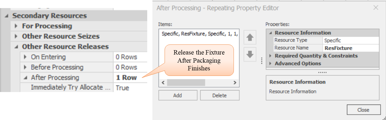
Figure 6.14: Releasing the Fixture
6.3.4 In order to “see” how the available capacity of the resource changes during the simulation, add a Status Label from the Animation section in the ribbon to make sure no objects are selected.72 When the status label is selected, the cursor can be used to draw a box onto the modeling canvas, as shown in Figure 6.15. Note that the expression gives the remaining capacity of ResFixture.
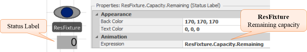
Figure 6.15: Adding a Status Label for Remaining Capacity
6.4 Changing Processing Time as a Function of the Size of the Queue
Suppose you find out that SrvPacker1 changes its processing time depending on the number currently waiting (i.e., the size of the queue). Specifically, the packer is only 80% as efficient when there is zero in the input buffer queue, 90% when there is one, and 100% for all others.
6.4.1 You need an “efficiency” table now to determine the processing time. This table can be modeled as a “Discrete Lookup” table in SIMIO (i.e., f(x)). From the “Data” tab, add a “Lookup Table” whose values are 0.8 for 0, 0.9 for 1, 1 for 2, and 1 for 100, as shown in Figure 6.16. Name the table LookupEfficiency.
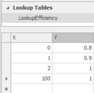
Figure 6.16: Lookup Table for Efficiency Calculation
Remember, the table gets interpolated for values between the discrete points. To access the efficiency based on the number waiting in the queue at the SrvPacker1, we will use the following expression:
LookupEfficiency[SrvPacker1.InputBuffer.Contents.NumberWaiting].
Notice that to access rows (i.e., indexing) into tables and arrays, SIMIO uses the [] notation rather than ().
6.4.2 We are planning on using the expression more than once in our model. Since the expression is very long and complicated, we will utilize SIMIO’s function expression creator to alleviate mistakes.73 From the “Definitions” tab under the Functions (f(x)) section, insert a new Function named FuncEfficiency. Set the Expression property to the appropriate value, as seen in Figure 6.17.
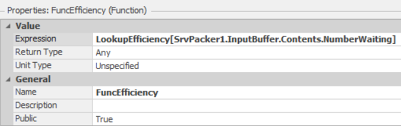
Figure 6.17: Specifying a SIMIO Function
6.4.3 Now, in the Processing Time property for the SrvPacker1, change the expression such that the Triangular distribution is divided by the efficiency function to get the actual processing time. The new expression is defined as the following.
Random.Triangular(3,5,8)/FuncEfficiency
6.4.4 We want to be sure our “efficiency” function is working correctly. To do that, we will use a SIMIO “Time Plot,” which you will find under the “Animation” tab in the ribbon. Use the following specifications for the plot, which are in the “Labels” and”Time Range” sections of the “Appearance” tab (see Figure 6.18).
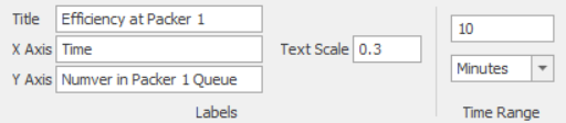
Figure 6.18: Setting the Properties of the Status Plot
Also, add the Expression property of the Status Plot that will be drawn, which is FuncEfficiency where the plot is given in Figure 6.19.
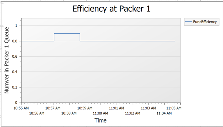
Figure 6.19: Efficiency Plot
6.4.4.1 Does it appear that the efficiency function is working?
_______________________________________________
6.5 Creating Statistics
Here, the SIMIO “automatic” statistics collection process may not provide the statistics that interest you. For example, we might want to know the time the boards and chips get from entry to exit, or we might want to know the average efficiency for SrvPacker1. Time in system or time in a “sub-system” is an example of “observation-based” statistics. Recall this type of statistic, which is referred to in SIMIO as a “Tally Statistic.” In the case of efficiency, its value is changing (discretely) with respect to time, and it is an example of what is generally referred to as a “time-persistent” or “time-weighted” statistic. In SIMIO, this type of statistic is a “State Statistic,” and since efficiency changes discretely, it is referred to as a “Discrete State Statistic.”74
6.5.1 Consider first the “state” statistic “efficiency.” We need to define a model-based (global) state variable for efficiency in collecting statistics on this characteristic. From the “Definitions” tab, select “States,” and in the “Discrete” section, click on “Real” to define a new state variable named GStaPacker1Efficiency.
6.5.2 To ensure that StaPacker1Efficiency is correctly monitored for its value by SIMIO, let’s modify the “State Assignments” in the SrvPacker1 Server. In particular, we will make the assignment On Entering the server and use the following assignments.
State Variable: GStaPacker1Efficiency
New Value: FuncEfficiency
6.5.3 Finally (this is the last step in collecting a state statistic), we need to define a “State Statistic.” New statistics can be defined from the “Definitions” tab but in the “Elements” section. Elements represent special objects that add modeling flexibility. Let’s call the new statistic the StateStatPacker1EfficiencyLevel and use GStaPacker1Efficiency as the State Variable Name, as seen in Figure 6.20.
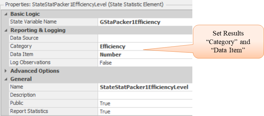
Figure 6.20: Setting a State Statistic
6.5.4 Save and run the simulation model for ten hours. Filter the results of the “Object Type” to “Model” to see the new statistic.
6.5.5 Next, let’s obtain the “time in system” statistics for the boards and chips to go from entry to exit. Although you might think you need to give some special instructions to SIMIO, this is a case where we can take advantage of the way SIMIO provides statistics. Recall that we automatically get “time in system” statistics on the entities exiting through a sink. We will exploit this modeling approach.
6.5.6 To obtain the statistics on the boards and chips, we can separate them and send them through separate exits (i.e., Sinks) – and do all this without changing the fundamental statistics. Our approach is shown below in Figure 6.21.
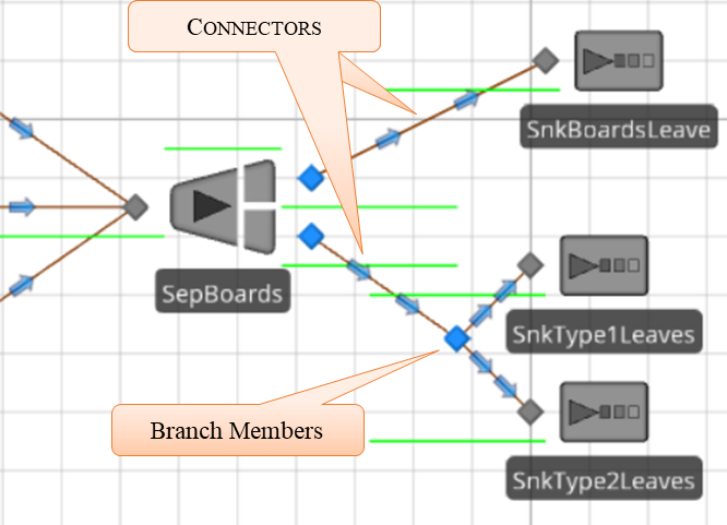
Figure 6.21: Separating Entities
The approach will substitute a Separator (from the [Standard Library]) for the original Sink and then branch the “parent” and “members” output to the appropriate Sink. One can either delete the Sink and add a Separator or right-click on the sink and select Convert To Type→Separator. The members get further branched to separate Sinks using a TransferNode. Connectors are used to connect objects, so no time is taken.
6.5.7 Again, using time paths, connects the packers to the input of the Separator, specifying the TimetoExit property as the travel time. The branching of members uses “Link Weight.” The Selection Weight property for the link connecting to the SnkType1Leaves Sink is ModelEntity.EStaChipType==1 while the Selection Weight property for the connector to the SnkType2Leaves Sink is ModelEntity.EStaChipType==2.
6.5.8 Run the model for 10 hours and answer the following questions.
6.5.8.1 How long are boards in the system from the time they enter to when they leave?
_______________________________________________
To add entities, drag ModelEntity from the [Project Library] panel.↩︎
Note memory boards are not ¼ meter thick but were made this thick to show a depth in 3-D view.↩︎
Select the EntMemoryChip ModelEntity and the click Symbols→3Additional Symbols→Add Additional Symbol button.↩︎
Select the 3-D view and color the sides of the new symbol as well.↩︎
Both the Model and ModelEntity can have a state variable named Color. The only difference is how they are accessed. Specifying Color will access the variable of the Model while ModelEntity.Color will access the entity’s variable.↩︎
The Discrete distribution must use the appropriate cumulative probabilities.↩︎
Combiners can match any entity, match members or match certain members and parents based on a criterion.↩︎
It is very easy to specify the Selection Goal property as the Selection condition. The selection condition property is an expression that has to evaluate to “True” before the item can be selected from the list (e.g., Server has not failed) as a possible choice.↩︎
Select all three time paths and then right click on the Travel Time property and select the new reference property TimeToExit.↩︎
Note that if a default value is not given, the simulation model may not run until you have set the property because it will be Null.↩︎
Remember that hitting the “h” key in the model window brings up instructions for moving around in 2D and 3D and also in manipulating objects. Hitting the “h” key again removes the instructions.↩︎
Recall the picture symbols start at zero which is why we need to subtract one.↩︎
Later chapters will go in more detail on the Resource object.↩︎
Note, a Resource is fixed object and cannot travel throughout the network. Other types of resources (i.e., Worker, Vehicle, and Entity) can be dynamic and move through out a network.↩︎
If we had selected the ResFixture first before inserting the status label, the label would be attached to the resource and therefore the expression would be just Capacity.Remaining. If we moved the Resource in the model the status label would move as well.↩︎
If we were to change the expression, it will only need to be modified in one place rather than in every location we used the direct expression.↩︎
Don’t confuse a “state variable” with a “state statistic”.↩︎