Simulation Modeling with Simio - 6th Edition
Chapter
9
The Workstation Concept: A Kitting Process
Often, a process, especially in a manufacturing environment, needs the ability to handle the situation of batching by processing an entity as though it were composed of several items or services one or more of the items at a time. Also, during the processing of the batches, we may need to consume or need materials to complete the processing. Materials are those items that are supplied to process and are directly required for the assembly/production of the finished item. A “bill of materials” typically determines what is needed for any operation. Materials are not objects but an inventory of items that can be consumed and replenished. While one can utilize entities and combiners to model this situation, it is not practical when you have millions of materials in the system. Also, processes often require a setup that may take time and resources or tear down/process finished time. In earlier versions of the book, the Workstation object was used to model this scenario, but that object has now been deprecated and is no longer supported by SIMIO117.
9.1 The Kitting Process
A kitting process constructs a “kit” from available components. Orders arrive at a kitting workstation in a Poisson stream with an interarrival time of three minutes, as seen in Figure 9.1. An order is for a particular number of identical kits to be produced. The kits are assembled from three components: one SubA subassembly, one SubB subassembly, and two Connectors – this is also referred to as a Bill of Materials (BOM). The assembly of each kit has a processing time described by a triangular distribution with parameters of (0.1, 0.2, 0.3) minutes. Only one kit can be assembled at the kitting station at a given time. Information about the kits produced and components used is needed to analyze the operation, and information on the processing of the orders is also desired.
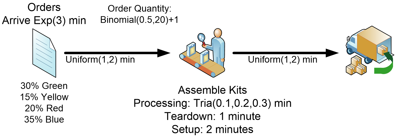
Figure 9.1: The Kitting Operation
Four types of kits are produced from the same BOM, representing the following colors: 30% are green, 15% are yellow, 20% are red, and 35% are blue. Following each order that is processed, it takes one minute to tear down for the next kitting order and two minutes to setup for the following order. This assumption will be changed later. Finally, the orders will be assumed to take between one and two minutes to arrive at the kitting workstation as well as to travel to the exit from the kitting workstation.
9.1.1 Create a new model that has one Source (SrcOrdersArrive), one Sink (SnkOrdersLeave), and one Workstation object (WrkKitOperation), as seen in Figure 9.2.
- Connect the objects using TimePaths that take the appropriate Uniform(1,2) minutes as the Travel Time property.
- The kits’ orders arrive with an Exponential(3) minute interarrival time with random stream one.
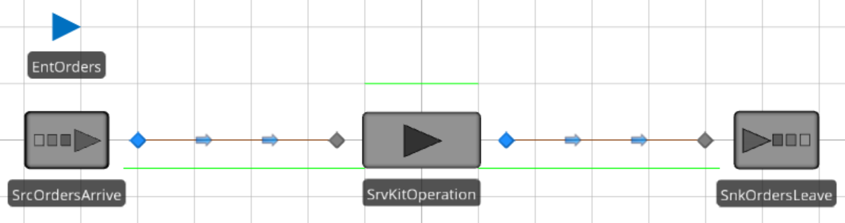
Figure 9.2: Kitting Operation Model
9.1.4 All of the SIMIO objects have specific built-in characteristics. Properties for an object (e.g., the initial number of in-system and maximum arrivals) are established at the time the object is created (usually at the beginning of the simulation) and cannot change during the simulation. State variables are characteristics that can change during the simulation. The SIMIO-defined Priority state variable119 is an example of a characteristic often used for ranking. In SIMIO, you can add your own properties and discrete state variables to objects.
Properties and States are added through the “Definitions” tab of an object. All objects in SIMIO can have their own Properties and States. A state variable defined in the Model will only have one value and can be thought of as having a global scope. Defining a state variable on the ModelEntity will allow each entity to have its own state variable value. Select the ModelEntity in the [Navigation] panel and select the Definitions→States section. Each kit order will have a different quantity of kits requested, and a state variable is needed to track this information.
- Notice that SIMIO already defines two state variables. SIMIO defines Picture as a Discrete Real State Variable representing which picture should be displayed to represent the entity. SIMIO also declares the Animation state variable, a String State Variable used to determine the type of moving animation the entity might do. The object also inherits other state variables from the parent object.
- You should add EStaOrderQuantity as a new Discrete Integer State Variable representing the number in the order, as seen in Figure 9.3
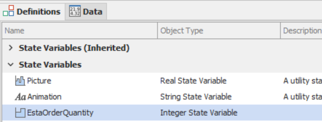
Figure 9.3: Kitting Operation Model
9.1.5 A table is needed to determine the percentage of time each type of order will occur and the symbol picture number. First, select the Model in the [Navigation] panel to return back to the simulation model. Let’s create the TableSymbol for the entity pictures, as seen in Figure 9.4 via the Data tab where the Symbol column should be an Integer Standard Property, the Percent could be an Integer, Real, or Expression property (i.e., numeric), and the Color is a String Standard Property.
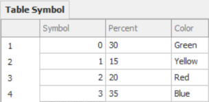
Figure 9.4: Order Type Symbol and Percentages
9.1.6 Next, the order type (i.e., yellow, red, etc.), the order quantity for the arriving order, and the correct picture will be specified using an Add-On process trigger. Select the SrcOrdersArrive and double-click the CreatedEntity Add-On process trigger property, creating the process named SrcOrdersArrive_CreatedEntity. After setting the table row, we can assign state variables to the incoming entities, as shown in Figure 9.5.120
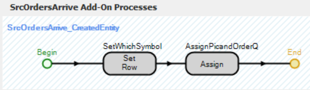
Figure 9.5: Setting the Row of the Data Table and Assigning the Picture
9.1.7 Use the Set Row process step to randomly assign a row of the TableSymbol Table to the entity, which will be used in the Assign step to specify the entity’s picture.

Figure 9.6: Steps for the OrdersArriveCreatedEntity Process
9.1.8 Next, assign the correct picture and the order quantity. You can do this in two different assignment steps or in one step using multiple rows by clicking the “0 Rows” button. You must add each assignment as seen below in Figures through Figure 9.9.
- Use the “Repeating Property Editor” to make multiple assignments, as shown in Figure 9.7.
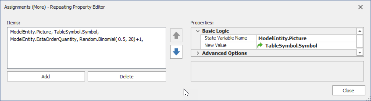
Figure 9.7: Making Multiple Assignments
- Set the picture to represent the symbol associated with the specified order type, as in Figure 9.8.121
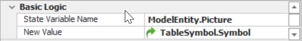
Figure 9.8: Picture Assignment
- Assign the order quantity from a Binomial Distribution as in Figure 9.9.
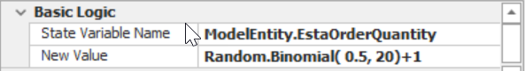
Figure 9.9: Order Quantity Assignment
9.1.9 To assist in validating the model, select the entity and set the Dynamic Label Text to ModelEntity.EstaOrderQuantity which will display the order quantity as the model is running.
9.1.10 The time needed to process each kit at the workstation follows a Triangular(0.1, 0.2, 0.3) minute distribution. However, the workstation has a teardown time of one minute and a current setup time of a specific two minutes. We need to incur the setup time before processing the batch, followed by a teardown time after the batch is completed. In this current scenario, we need to add the setup and teardown times into the processing times.
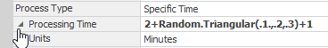
Figure 9.10: Adding in the Setup and Teardown Time
9.2 Modeling Batching, Setup, and Teardown Times
A service activity may be composed of several tasks rather than a simple processing time. For example, the kitting of an electronic product may employ a sequence of tasks to complete the kit (i.e., Setup, Processing, and Teardown). Likewise, an inspection may require several tests at the inspection station. Often, the details in these types of operations can be conveniently summarized by their processing time. There are, however, instances when the processing time needs a composition of a set of interrelated tasks. SIMIO, therefore, recognizes two types of processing stations within a Server, which are referred to as Process Types. Specifically, the alternative specifications are “Specific Time” or “Task Sequence”. We have only modeled using the Specific Time, the default value. A task sequence refers to a network of tasks ordered by precedence. For example, you need a nurse to take vitals and information, then you need to see the doctor, potentially followed by more nurse visits. This would be harder to handle using one Server. When more details about a process needed to be included in the model, the model was extended with more objects (i.e., additional servers were inserted). Using the Task Sequence process type, details about processing can be incorporated into a set of task sequences within a single Server rather than modeled with a series of Servers.
While the current scenario is a very simple process, separating out the setup and teardown steps into separate individual tasks, as seen in Figure 9.11, will allow more flexibility. For example, the setup and teardown may require an operator, sequence-dependent setups, set of tools, etc., to perform the task.
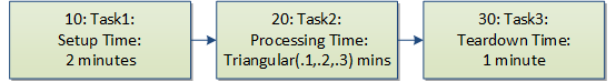
Figure 9.11: Modeling Setup, Processing, and Teardown as Independent Processes
9.2.1 Change the Process Type of the SrvKitOperation to “Task Sequence.”
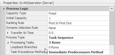
Figure 9.12: Specifying the Task Sequence Process Type
9.2.2 We need the ability to specify the sequence order of a set of tasks (i.e., how do we indicate the precedence network). There are three different methods of specifying the precedence network, as outlined in Table 9.1. A more complicated task sequence diagram of the Bank Teller will be explored in detail in a later chapter. Change the Task Precedence Method to the Immediate Predecessors Method, which allows us to specify the predecessor tasks that must all be completed before the current task can start to be executed.
| Process Type | Description |
|---|---|
| Sequence Number Method | Expression represents the time needed for the task to complete. |
| Immediate Predecessors Method | Using the Immediate Predecessors property within each task, you specify all the tasks that need to precede this task before it is started (e.g., 10 or 10, 20). |
| Immediate Successors Method | Using the Immediate Successors property within each task, you specify all the tasks that need to start after this task is completed (e.g., 20 or 20, 30). |
9.2.3 Click on the Processing Tasks property additional items button […] and add the three tasks using the specifics in Figure 9.13. The ID Number for each task must be a unique identifier that will be utilized to specify the Immediate Predecessors. Leave the Immediate Predecessors property blank if there are no predecessors, as is the case for the Setup Time task. For the batch time task, the preceding task is the setup time (i.e., identifier 10), while the batch time task (i.e., identifier 20) needs to be finished before starting the teardown task as specified.
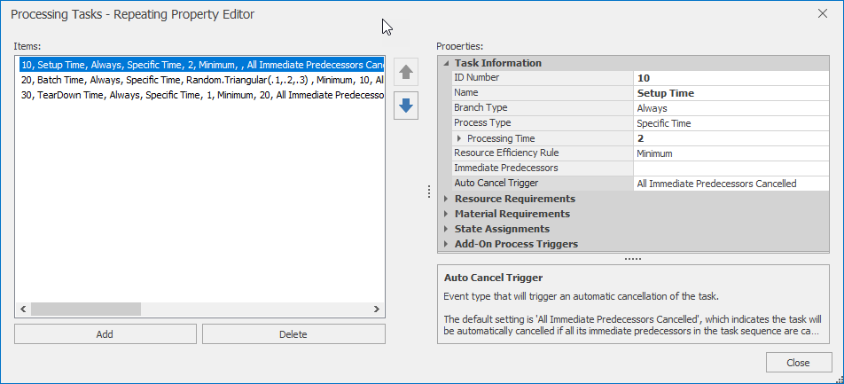
Figure 9.13: Specifying the Three Tasks
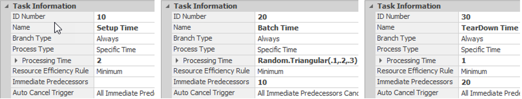
Figure 9.14: Specifying the Setup, Batch, and Teardown Time Tasks
9.2.4 Save your model and run the model for eight hours.
9.2.4.1 What is the average flow time for the orders?122
_______________________________________________
9.2.5 Up to this point, the processing time for each order was the same regardless of the order quantity. The processing time for a batch of parts to be processed individually is the sum of a series of independent processing times. One may think to model this situation is to sample from the random distribution once and then multiply by the order quantity (i.e., quantity * triangular (.1,.2,.3)). Even though the mean will be equal, the variation will be much larger than if we summed up multiple random distributions. See Appendix A, section eight, on modeling the sum of N independent random variables. Change the processing time of the batch task using the Math.SumofSamples function will sample from the distribution EstaOrderQuantity a number of times and sum the values.
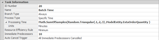
Figure 9.15: Handling the Batching of the Kits
9.3 Sequence-Dependent Setup Times
Currently, the setup time is a constant of two minutes, regardless of the sequence of colors. Whenever the kitting workstation must change from one color to another, a set-up time depends on the color type that preceded the current order. The changeover time is shown in Figure 9.16. Let’s add the sequence-dependent set-up times to our model.
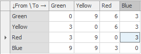
Figure 9.16: Changeover Set-up Times (From/To) in Minutes
Under the TaskSequence properties, we specified the constant two-minute set-up time for the kitting operation using “Specific Time” as the Process Type with the Specific constant set-up (e.g., two minutes for the kitting operation), as seen in Table 9.2. But before we can use sequence-dependent set-up times, we need to know how the changeover times can be incorporated into the SIMIO model by using a changeover logic element and changeover matrix.
| Process Type | Description |
|---|---|
| Specific Time | Expression represents the time needed for the task to complete. |
| Process Name | Specify a process that will be executed when the task starts. The task will finish once the process has finished executing. |
| SubModel | Allows you to create a different model within the current facility window. When the task starts, an entity of a specified type will be created and sent to the starting node of the submodel. You can save a reference to the original entity to pass information to the created entity. The task finishes once the created entity is destroyed by the submodel. |
| Sequence Dependent Set-up Time | Allows you to specify a sequence-dependent set-up logic. |
9.3.1 First, a List of identifiers is needed that can be used to create the changeover table (matrix), which, in this case, is a List of Strings. Under the “Definitions” tab, insert a List of Strings named LstColors. The contents of the LstColors list would correspond to our symbol colors: “Green,” “Yellow,” “Red,” and “Blue,” as seen in Figure 9.17. These must be put in this order to correspond to the symbols (0, 1, 2, and 3).
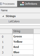
Figure 9.17: List of Colors
9.3.2 Now, in the “Data” tab, add a Changeovers matrix (this is a “from-to” matrix) named Changeover and use the LstColors list for the associated list. Change the unit of time to Minutes and enter the values into the matrix from Figure 9.16.
9.3.3 Next, from the “Definitions” tab, insert a Changeover Logic Element named ChangeoverKitLogic, as seen in Figure 9.18.
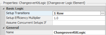
Figure 9.18: Inserting a Changeover Element
| Changeover Properties | Description |
|---|---|
| Set-up Transitions | Allows one to specify multiple set-up transitions either via change over the matrix or other criteria. |
| Set-up Efficiency Multiplier | It can be used to increase or decrease the total time taken for a set-up by either a constant or expression. It can be used to model variability in a constant set-up time. |
| Assume Concurrent Set-ups IF | An expression is evaluated before the change over time is calculated. If the condition is true, then the total time for the changeover will be the longest of several different set-up transitions. If it is blank or false, the total changeover time will be the sum of all the different set-up transitions. |
9.3.4 Click on the Set-up Transitions … to invoke the repeating property editor to specify how to sequence-dependent transitions. Next, specify the setup time logic, as seen Figure 9.19. The assigned symbol number will be used to determine the transition from the previous symbol, which is stored automatically by SIMIO.
- Operation Attribute: TableSymbol.Symbol
- Use Changeover Matrix property: True
- Changeover Matrix Name: Changeover
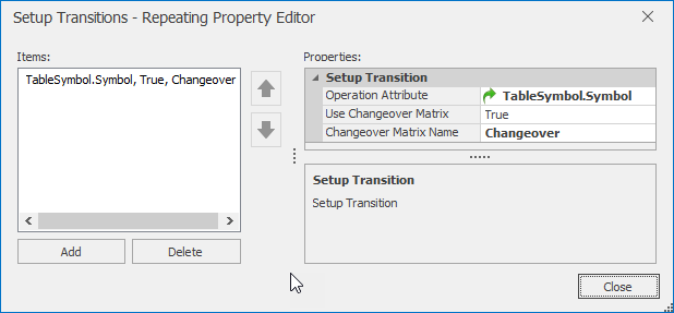
Figure 9.19: Specifying the Transitions as a Changeover Matrix
9.3.5 We can now finish by specifying the set-up time task sequence to use the ChangeoverKitLogic element. Select the SrvKitOperation and specify the other elements of the Process Logic for the Task Sequence, as seen in Figure 9.20.
- Process Type property: Sequence Dependent Set-up
- Changeover Logic Name: ChangeoverKitLogic
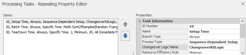
Figure 9.20: Task Changeover Properties
9.3.6 Recall the Server can be in several different resource states, including starved (i.e., idle), processing, performing a set-up, etc. To see all nine possible server states, click the SrvKitOperation and click the “Active Symbol” button. To see the percentage in these “resource” states evolve while the simulation is running, add a “Status Pie” from the Animation tab. Specify the Data Source property SrvKitOperation.ResourceState.123
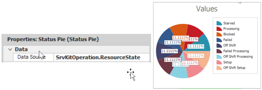
Figure 9.21: Server Status Pie Chart
9.3.7 Save and run the simulation with animation for an hour. Then, run it in fast-forward mode for two, four, and eight hours. After eight hours, answer the following questions.
9.3.7.1 What is the time in the system and the average set-up time of the server?
_______________________________________________
9.4 Sequence-dependent set-up Times that are Random
The previous section utilized the ChangeOver matrix to handle sequence-dependent set-up times. However, the matrix is limited to only constant/deterministic times and cannot handle the case when the set-up times have variability associated with them (i.e., random distributions). Since SIMIO’s ChangeOver matrix cannot utilize distributions as the sequence-dependent set-up times, we will handle this manually using related data tables. Similar to previous examples, a child table will be used to define the set-up times for a particular part.
9.4.2 First, we need to declare the relationship (i.e., primary key) for the parent table. From the Data→Tables section, select the column named Color in the TableSymbol table. Click the Set Column as Key button and fill in the field’s values, as seen in Figure 9.22.124
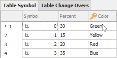
Figure 9.22: Adding the Color Field as the Primary Key
9.4.3 Insert a new Data Table named TableChangeOvers, as seen in Figure 9.23, which will be the child table.
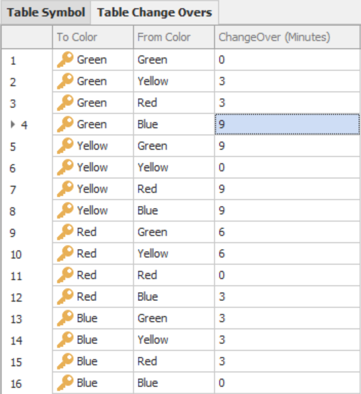
Figure 9.23: Creating the Sequence Dependent Set-up Times Table
9.4.4 From the Add Column section, select the Foreign Key to insert the To Color column. Set the Table Key property to TableSymbol.Color which will link the parent to the child changeover’s table.
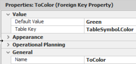
Figure 9.24: Adding the “To Color” Child Foreign Key
9.4.5 Insert a Standard String Property named From Color and an Expression Standard Property named ChangeOver. Make sure to set the Unit Type property to “Time” and the Default Units to “Minutes.” Since this column is an Expression property column, we can specify any SIMIO expression, including sampling from a random distribution.
9.4.6 Insert the values from Figure 9.23, which replicates the previous section’s set-up times.
9.4.7 When the EntOrders are created, they are assigned a row to the TableSymbol (see Figure 9.5), which was used to determine the picture. Now, they will also be assigned the related portion of the TableChangeOvers, as seen in Figure 9.25, if the new order was “Red.”
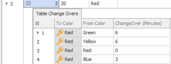
Figure 9.25: Related Records in the ChangeOver Table Associated with Red Orders
9.4.8 If the new order “Red” is next to be kitted and the previous order was “Yellow,” then the set-up time should be six, which is associated with the second row of the related table, as seen in Figure 9.25. However, we need to know which color was processed last. From the “Definitions” tab, insert a new Model Discrete Integer State variable named GStaPreviousColor with a default value of “1,” indicating the last color processed.
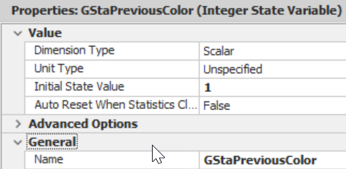
Figure 9.26: Insert a State Variable to Keep Track of the Last Order Processed
9.4.9 Select the “Set-up Time Task” from the Task Sequences of the SrvKitOperation. Under the State Assignments property, set the GStaPreviousColor to the current symbol plus one, which will be used for the next order. The symbols range from zero to three, but table rows start at one. Change the Assign When properties to “Finished Task” will make the assignment after the set-up task finishes.
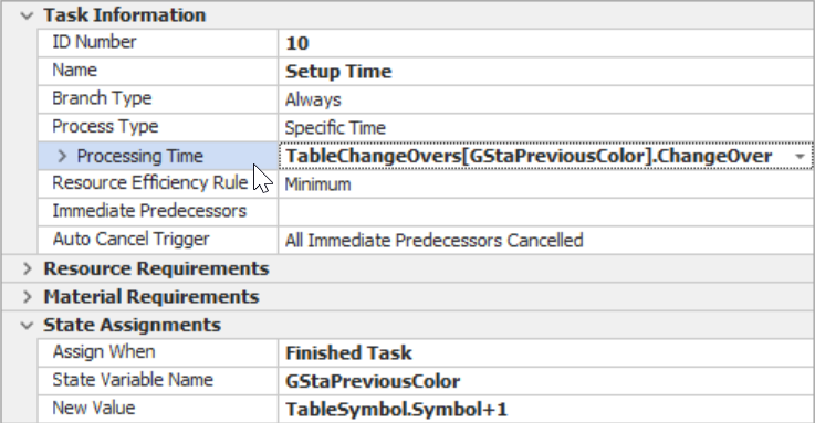
Figure 9.27: After Set-up is Completed, Set the Previous Color
9.5 Using Materials in the Kitting Operation
SIMIO can keep track of raw materials that must be consumed, as specified in the “bill of materials” needed to create a part or complete an assembly. If the raw material is unavailable, parts (i.e., entities) cannot be processed and will wait until the required materials become available. These can be used to track inventories much easier than if you were just using state variables. In this example, each kit needs three materials in order to be produced.
9.5.1 Return to the model from Part 9.3 of this chapter and save it as a new model.
9.5.2 First, we need to declare the existence of raw materials that make up a kit and the Bill of Materials that specify the number of each raw material type needed to make a kit. Five new Material “Elements” need to be defined via the Definitions→Elements→Workflow section, as seen in Figure 9.28.125
- Create MatSubA, MatSubB, and MatConnectors as materials types, all with Initial Quantities of zero, which will be changed shortly.
- Next, create a MatBOMKits as a Material element, but using the BillofMaterial Repeating Property Editor as shown in Figure 9.28 to define what materials make up this product (i.e., one MatSubA and MatSubB and two MatConnectors).
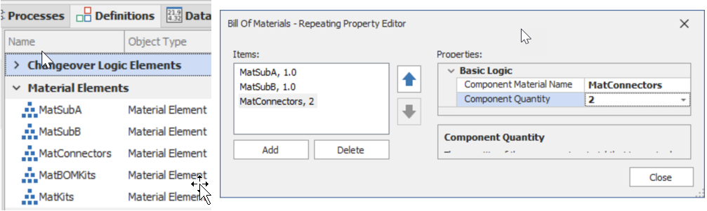
Figure 9.28: Five Materials and the Bill of Materials for the MatBOMKits
- Finally, create MatKits as the last “Material” element (with an Initial Quantity of 0) which will represent the finished product produced from the raw materials in the bill of materials.
9.5.3 Since the initial inventory is a fixed characteristic of our model and only needs to be initialized at the start of the simulation, here is an ideal place to use a SIMIO Model “property.” From the Definitions→Properties” section, add new properties to objects. Create three new “Standard Real or Expression Properties” named InitInvA, InitInvB, and InitInvC. Place all of these properties into a new InvModel Category. The first time, the new category name (InvModel) needs to be typed into the window. You can select the category from the drop-down menu for the next two properties.

Figure 9.29: Creating Initial InventoryProperites
9.5.4 Return to the material “Elements” and set the Initial Quantity property for each of the three materials (i.e., MatSubA, MatSubB, and MatConnectors) as a reference property to the previously defined properties. Remember, this is done by right-clicking on the drop-down arrow and selecting the referenced property, as seen in the figure below.
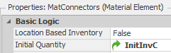
Figure 9.30: Specifying the Initial Inventory of Materials using the Inventory Properties
9.5.5 We can use the materials as part of the definition of the task sequences or use a process to consume and produce materials. Now return to the model under the Facility tab, and for the Server SrvKitOperation Task Sequences, fill in the Materials Requirements properties (i.e., Action Type, Material Name, and Quantity property under the Required Quantity & Constraints) as seen in Figure 9.31. The Quantity property specifies how many materials to consume or produce. We will use the “Batch Time” task to consume materials based on the bill of materials and the “TearDown Time” task to produce the kits.
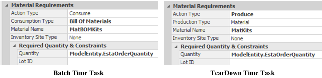
Figure 9.31: Other Material Requirements for a Task Sequence
9.5.6 To access the new Model properties we created, click on the Model “Properties” (by right-clicking the “Model” object in the [Navigation Panel]).126 In the Controls →InvModel section set the values of the InitInvA to 100, InitInvB to 100, and InitInvC to 200.
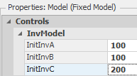
Figure 9.32: Setting Model Properties
9.5.7 Save and run the new model for eight hours, observing the statistics. While you may want to run it for a while looking at the animation, you will need to fast-forward to the end to get the results.
9.5.7.1 After looking at the Kits produced, do you have concerns about the model specifications?
_______________________________________________
9.5.7.2 How many kits were produced in the eight hours?
_______________________________________________
9.6 Raw Material Arrivals during the Simulation
Instead of material being available for the entire eight-hour day at the beginning of the simulation, the raw materials will be scheduled to arrive every two hours, beginning at time zero. When the stock arrives, the inventory is returned to a target stock level – implementing an “order-up-to-inventory policy.” How would this be modeled in SIMIO?
9.6.1 Save and run the model for eight hours using initial inventory quantities of 1000, 1000, and 2000 for SubA, SubB, and Connectors (specified in the “Model Properties”).
9.6.2 Now, let’s implement a replenishment system in which a stocker comes by the kitting station every two hours, beginning at time zero, and fills up the stock for MatSubA, MatSubB, and MatConnectors to particular quantities.
9.6.3 Add three order quantity properties for the model under the Definitions tab: OrderQtySubA, OrderQtySubB, and OrderQtyConn. Each of these properties should be an Integer Data Format added to the InvModel category, as shown in Figure 9.33. These properties will be used as the order-up-to quantities that the stocker uses to replenish the raw material inventory.127
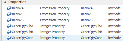
Figure 9.33: Order Quantity Properties
9.6.4 Under the Definitions→Elements section, add aTimer element that will fire an event based on a time interval (a “timer event” will be an interruption in the simulation that allows a process to execute). See Figure 9.34.
- Start the timer at time 0.0 (i.e., Time Offset property should be 0), meaning the first event fires at time zero, and it then should “fire” an event every two hours (i.e., Time Interval should be “2”).
- Name the timer TimerStockerArrives.
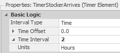
Figure 9.34: Timer for Stocker Arrivals<
9.6.5 Under the “Processes” tab, create a process named RespondtoTimerEvent that will respond to the timer event when it expires, as seen in Figure 9.35.
- Triggering Event property: TimerStockerArrives.Event
- Add an Assign step that makes the following assignments to the process, which always makes the quantity available equal to the order quantity (i.e., order-up-to policy).128
MatSubA.QuantityInStock = OrderQtySubA
MatSubB.QuantityInStock = OrderQtySubB
MatConnectors.QuantityInStock = OrderQtyConn
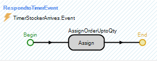
Figure 9.35: Process Used to Respond to the Timer Event
9.6.6 Now, in the “Model Properties,” set the initial values of the raw materials InitInvA, InitInvB, and InitInvC elements to zero since the first TimerStockerArrives event occurs at time 0.0 and will replenish the stock at the beginning of the simulation. Set the order quantities for OrderQtySubA, OrderQtySubB, and OrderQtyConnectors to 250, 250, and 500, respectively.
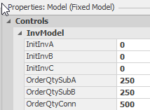
Figure 9.36: Setting the Model Properties for Order Quantities and Initial Inventory
9.7 Implementing a Just-In-Time Approach
The previous example assumed a stocker would come by (exactly) every two hours and replenish the inventory up to a certain level (i.e., an order-up-to policy). However, the company is moving toward a more Just-In-Time (JIT) type of operation. They have a supplier that is located a distribution warehouse very near the plant and will respond to orders very quickly. The company has implemented a monitoring system such that when the inventory drops below a certain threshold (i.e., reorder point), an order is placed to the supplier, who can supply the products within an hour.
9.7.1 Save the current model to a new name. You need to delete the TimerStockerArrives Timer Element and the RespondToTimerEvent process or disable the Timer by setting the Initially Enabled property to False under the General properties of the Timer.
9.7.2 Add a new Sink named SnkInventory. Position it underneath the Kit Operation, which will be used to model the arrival of new raw materials (MatSubA, MatSubB, and MatConnectors).
9.7.3 Add three reorder point properties for the model under the “Definitions” tab named ReorderPTSubA, ReorderPTSubB, and ReorderPTConn. Each property should be an “Integer” Data Format added to the InvModel category. These properties will be used as the reorder points for the JIT system to replenish the raw material inventory.
9.7.4 Go to the “Definitions” tab and add three Monitor elements underneath the”Element” section named MonitorA, MonitorB, and MonitorC. A monitor element can be used to monitor the value of a state variable when it changes value or when the state variable crosses some threshold (either from above or below). Refer to Figure 9.37 for the monitor properties for MonitorA.
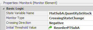
Figure 9.37: Monitor Properties
The following settings for MonitorA will monitor the SubA inventory level.
- Monitor Type should be CrossingStateChange.
- Crossing Direction should be Negative (i.e., 5 to 4 will fire an event if 4 was the threshold).
- The Threshold Value should be set to the new reference property named ReorderPTSubA.
- The Monitor can cause a process to fire just as the Timer element did, but we will not use this feature this time.
9.7.5 Repeat the same process for raw material MatSubB and MatConnectors material using ReorderPtSubB and ReorderPtConn reference properties, respectively.
9.7.6 Add three Sources (i.e., suppliers) named SrcSupplierA, SrcSupplierB, and SrcSupplierC, which will send the various raw materials to the kitting operation, as seen in Figure 9.38.
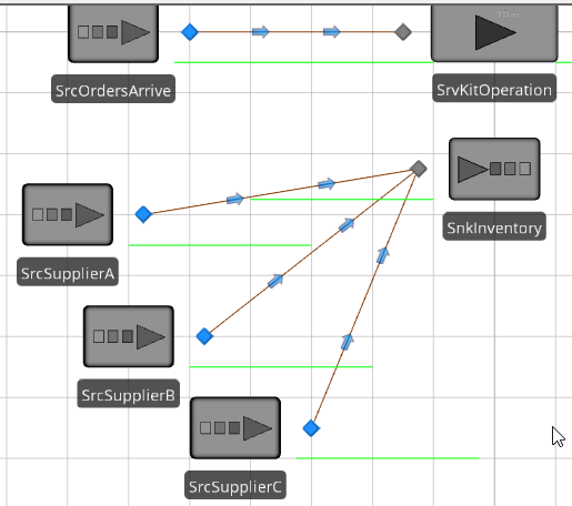
Figure 9.38: Supplier Sources
- Assume that it uniformly takes between 50 and 65 minutes for the raw materials to be delivered between the sources and the SnkInventory sink (this is modeled as the Travel Time property of a TimePath).
- Name each TimePath as TPA, TPB, and TPConn for the three TimePaths, respectively.
- Set the Arrival Mode property of the suppliers to On Event and the Event Name to MonitorA.Event, MonitorB.Event and MonitorC.Event respectively for each of the three sources as seen for SrcSupplierA in Figure 9.39. Each source will create an entity when its monitor event fires and sends the replenishment entity to the kitting operation.
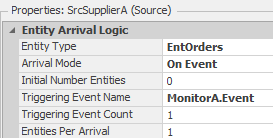
Figure 9.39: Utilizing an On Event Arrival Process
9.7.7 When the raw material reaches the end of the path, you need to increment the current quantity by the appropriate order quantity using the ReachedEnd add-on process trigger for each of the three TimePaths. A Tokenized Process will be used instead of three separate processes. From the Definitions→Token section, add a custom Token named TknReplenish. For this Token, add a “Material Element Reference” state variable named TStaWhichMaterial to reference the correct material and an “Integer” state variable TStaQuantity, as seen in Figure 9.40
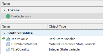
Figure 9.40: Adding the Custom Token to Pass in the Material and Quantity
9.7.8 From the Processes tab, insert a new process named Replenish, which uses the TknReplenish and specifies two Input Arguments properties named MaterialToProduce and QuantityToProduce, as seen in Figure 9.41.
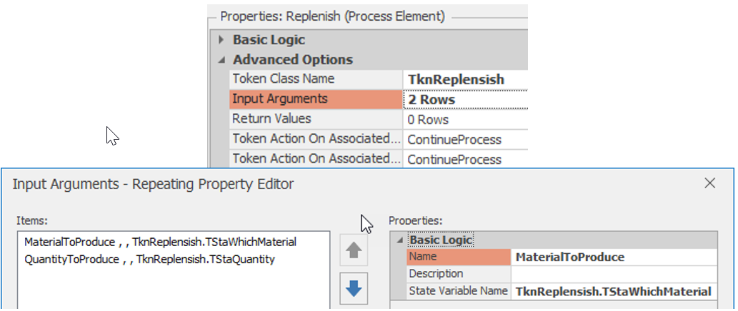
Figure 9.41: Specifying the Custom Token and Input Arguments
9.7.9 Insert a Produce step (see Figure 9.42), which will be used to add the order quantity to the particular material passed to the process. You will need to type the material name property value TknReplenish physically.TStaWhichMaterial directly rather than selecting it from the drop-down list.
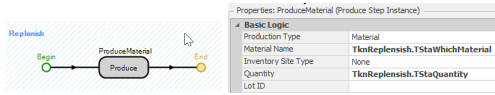
Figure 9.42: Incrementing the Quantity Available
9.7.10 For each of the Timepaths (i.e., TPA, TPB, and TPC), specify the Replenish process as the ReachedEnd Add-On Process Trigger property using the appropriate material and order quantity. Figure 9.43 shows the example for TPA using material MatSubA and quantity OrderQtySubA.
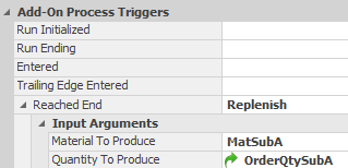
Figure 9.43: Using the Tokenized Process for Material A Production TPA Path
9.7.11 In the Model properties, set the initial values of the raw materials MatSubA, MatSubB, and MatConnectors elements back to 250, 250, and 500 since the replenishment is being triggered. Set the reorder points and order quantities to the values provided in Table 9.4.
| Raw Material | Reorder Point | Order Quantity | Initial Inventory |
|---|---|---|---|
| SubA | 125 | 200 | 250 |
| SubB | 125 | 200 | 250 |
| Connector | 250 | 400 | 500 |
9.7.12 While the simulation is running, we would like to display the available quantities of each of the three raw materials: MatSubA, MatSubB, and MatConnectors with either status labels or table.
- Add six “Status Labels” from the Animation tab that will display the available quantities of each of the three raw materials: MatSubA, MatSubB, and MatConnectors. The first three status labels are just text, with the other three labels having an expression, as seen in Figure 9.44, which will display the QuantityInStock for each material.
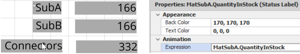
Figure 9.44: Status Labels and the Expression for the Status Label
- If you have many items to display or they change often, use a “Status Table,” which uses a data table to populate the statuses automatically. First, from the Data tab, insert a new table named TableLabelOutput, as seen in Figure 9.45, where the Material column is a String Standard Property, and the In Stock column is an Expression Standard Property. Add a “Status Table” from the Animation tab specifying the TableLabelOutput as the Table Name value.
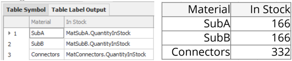
Figure 9.45: Using a Status Table vs Individual Labels
9.8 Commentary
- This is one of the most interesting chapters in that it illustrates how to model what would be considered a very complex operation composed of inventory concerns and supply chain issues. It’s a powerful lesson, and the topic of inventory and supply will be considered in additional chapters, along with some of the SIMIO features illustrated here.
- Task Sequences, Materials, and Bill of Materials is an extremely powerful modeling concept with numerous applications.
You can access deprecated objects by right-clicking in the Standard Library area.↩︎
Symbol numbers are in parentheses.↩︎
There is an entity property called Initial Priority, which initializes the Priority state variable.↩︎
Instead of using an add-on process trigger, the On Created Entity Table Reference Assignment could have been used to do the same thing along with the Before Exiting State Assignments.↩︎
The Picture state variable sets the symbol associated with the object in this case the ModelEntity.↩︎
You may notice the answers to these two questions do not match the previous answers. This is due to the random number sampling order changing (i.e., different random numbers). If you run an experiment with multiple replications, the mean answers would be statistically the same. If one wanted to control random numbers (i.e., common random numbers), then we would need to set specific unique random streams for each distribution (e.g., Random.Exponential(3, 1), which specifies the use of random stream number one for the distribution.↩︎
Note, if you select the SrvKitOperation object first and select the “Status Pie” from the “Associated Animation” tab, you will only need to specify ResourceState.↩︎
We could have used the Symbol field as the primary key, but this will make the setups easier to visualize in the related table.↩︎
Elements are objects that represent things in a process that change state over time (e.g., TallyStatistic, StateStatistic, Timer, etc.)↩︎
Note you can change the name of the fixed model as well as set other model properties.↩︎
Create one of the properties with the correct category and name. Then copy, paste it and change the name appropriately.↩︎
SIMIO provides a Produce step that essentially does the same thing and a Consume step which would perform a subtraction, but the logic using an Assign step seems just straight forward. In this example, you would add three Produce steps that would produce for example OrderQtySubA – MatSubA.QuantityAvailable.↩︎