Simulation Modeling with Simio - 6th Edition
Chapter
3
Modeling Distance and Examining Inputs/Outputs
This chapter aims to model people arriving at an airport and going through the check-in process. In the first phase, we are only concerned with the amount of time it takes the passengers to reach the security checking station so we can determine the needed number of workers at a check-in station. Passengers arrive at the terminal and proceed to the check-in process to get their tickets. After check-in, the passengers proceed to the security checkpoint.
Passengers arrive according to an exponential distribution with an average of one arrival per minute. Passengers walk to the check-in station at a rate uniformly distributed between two and four miles per hour. Passengers travel 50 yards from the terminal entrance to the check-in station. Following check-in, they must walk 65 yards to the security checkpoint, as seen in Figure 3.1. The check-in station currently has four people to process customers who wait in a single line. The check-in process takes between two and five minutes, uniformly distributed. The simulation model needs to be run for 24 hours.
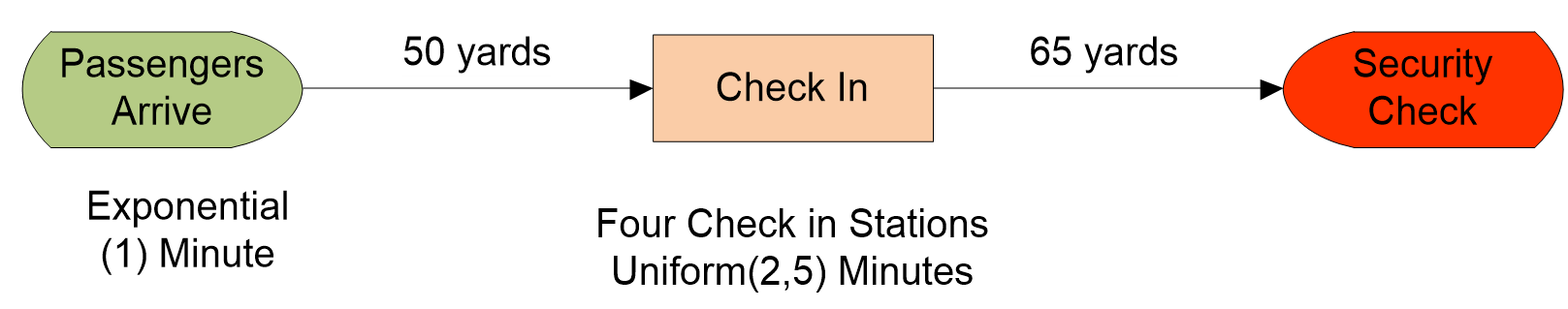
Figure 3.1: Airport Check-in Process
3.1 Building the Model
3.1.2 Insert a Source named SrcPassengersArrive, a Server named SrvCheckIn, and a Sink named SnkSecurity from the standard library to the Facility window and connect them using a path linkage (all of this can be done using the “Add-In” section on the “Project Home” tab).15
3.1.3 Click and drag an entity from the ModelEntity from the Facility window into the [Project Library] panel onto the Facility window. Also, change the name from DefaultEntity to EntPassenger. Change the passenger symbol to a person from the people library (either animated or static – we will use the static people pictures(“Woman1”) this time so you can see how they behave during the simulation).16
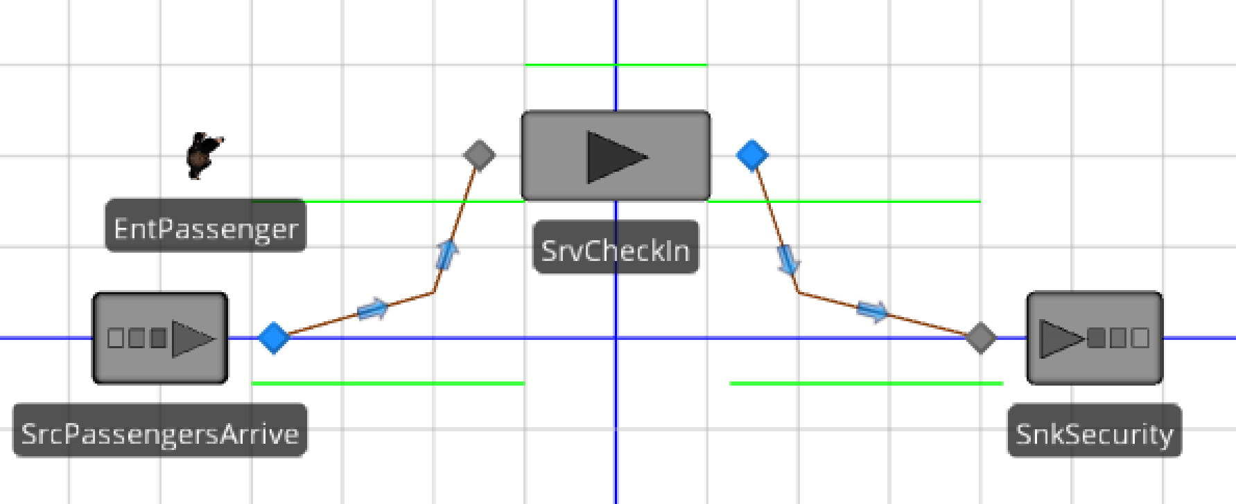
Figure 3.2: The Basic model
3.1.4 Random.Uniform(2,4) miles per hour in the EntPassenger o bject.Set the Interarrival Time property, Random.Exponential(1) minutes in the SrcPassengersArrive Source object. Set the Processing Time in the SrvCheckIn object to be Random.Uniform(2,5) minutes and make sure to set its initial capacity to four.
3.1.5 For the two paths, change the Drawn to Scale property of both paths to “FALSE” and set the correct distances for each. Recall that the path from arrival to check-in is 50 yards, while the path from check-in to security is 65 yards.
3.1.6 Run the simulation and observe the behavior of the “passenger” and the changing color of the check-in.
3.1.6.1 What does the passenger look like as they “move”?
_______________________________________________
3.1.6.2 What color is the check-in when it is idle and when it is busy?
_______________________________________________
The symbol colors for the check-in can be seen by clicking on the Active Symbol (1 of 9) down-arrow in the Additional Symbols section. It shows the nine “default” states of the server.
3.2 Using the 3D Warehouse
Although we have a working model, let’s change the server symbol. You can change the symbol of any entity or object by clicking the entity or object and changing it to some of the preloaded symbols in SIMIO. Alternatively, you can download new symbols from the Trimble 3D Warehouse™, or if you have symbols17 already on your computer, you can import them into this model.
3.2.1 To employ new symbols, select the SrvCheckIn object and click one of the nine choices among Project Symbols for the Server. The Trimble 3D Warehouse™ should pop up when you click the “Go to 3D Warehouse” button, which will allow you to search for any symbol you want (e.g., try searching for “Airport Baggage” after selecting the Models tab). Once you find a suitable model, click the “Download” button on the top right, and the Sketchup™ model will download.
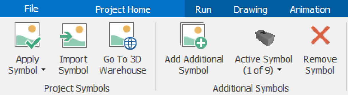
Figure 3.3: Downloading and Importing 3D Symbols
3.2.2 Next, click the “Import Symbol, and import the downloaded 3D Sketchup model. SIMIO will open an”Import” window where you can change some of its properties, such as size and orientation, before inserting the symbol into your model, as seen in Figure 3.4. First note: you can view the downloaded symbol in 2D and 3D. Also, it has length, width, and height that can be specified (in meters). A size “hint” is shown relative to a person so that you can modify the size based on that. Finally, you can rotate the symbol so it has the proper “orientation.” Change the Length to 5.2 m to make the symbol smaller and rotate the object by -90 degrees so the forward is the direction in which the entities will enter the object from the left.
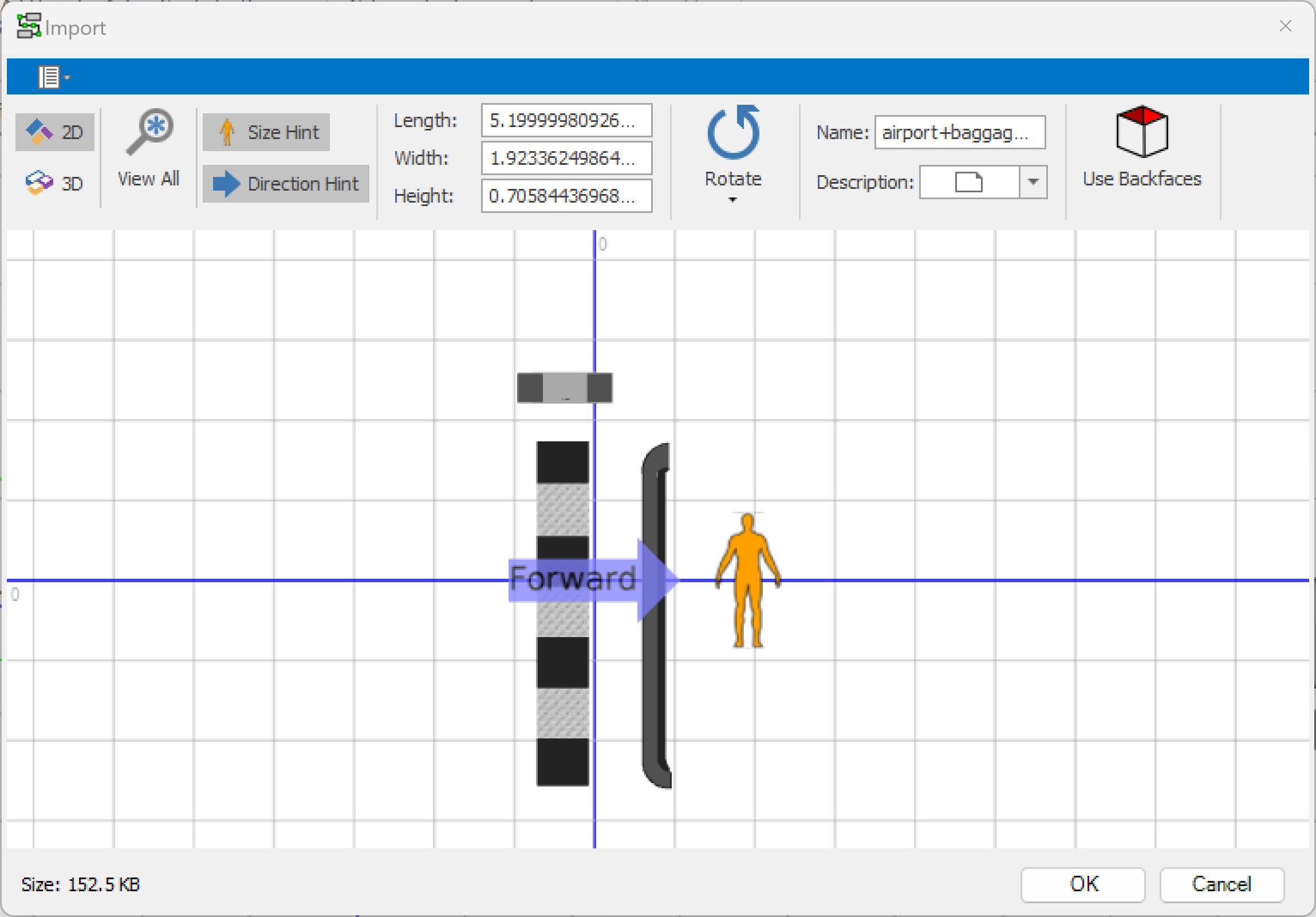
Figure 3.4: Import Trimble 3D Symbol Model
3.2.3 Position the baggage SrvCheckIn object so that the Input BasicNode, the InputBuffer queue, and the Processing queue symbols give the appearance of check-in at an airport, as shown in Figure 3.5.
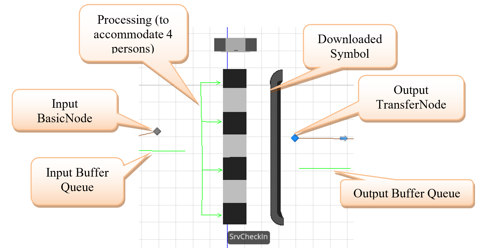
Figure 3.5: Baggage Check-In
3.2.4 Run and adjust the animation (in 2D and 3D). Lengthen the Processing queue of the SrvCheckIn server and modify the symbol using “Oriented Point” to show that up to four people can simultaneously be in-process at the check-in station by adding two additional vertices, as seen in Figure 3.6.
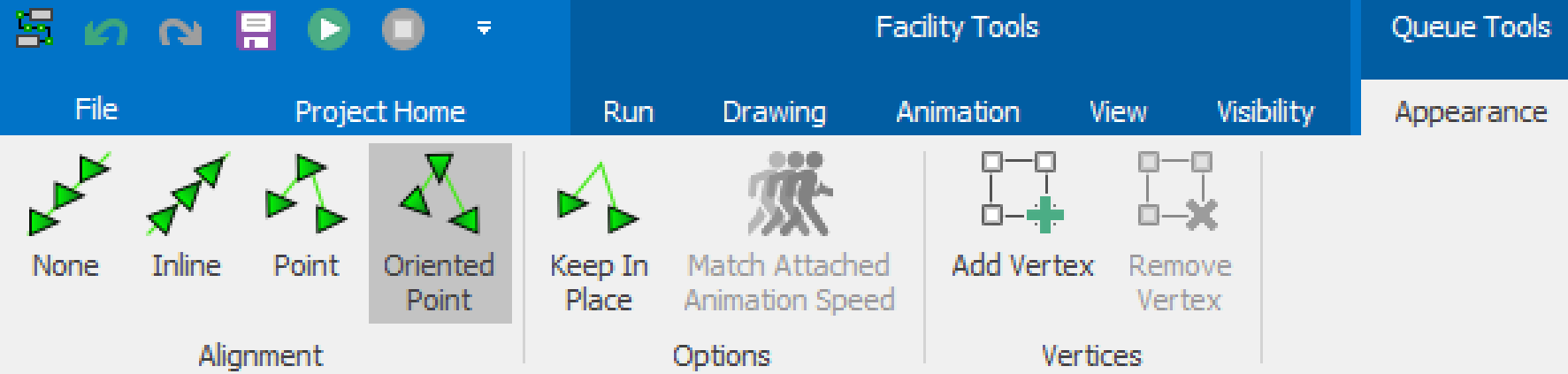
Figure 3.6: Modifying the Properties of the Queues
3.3 Examining Model Input Parameters
Before looking more closely at the output, let’s re-examine our “input.” Using input parameters, we can use SIMIO to understand our assumptions about the interarrival time and processing time. Using input parameters instead of directly specifying the expressions allows one to use the same random expression across multiple objects (i.e., five machines all have the same processing time) but, more importantly, will enable response sensitivity and sample size error analysis to be performed.
3.3.1 Click the “Data” tab and select the”Input Parameters” icon in the View panel on the left. Three types of input parameters can be defined: Distribution, Table Value, and Expression.18
3.3.2 Click on “Distribution,” which means we are interested in a statistical distribution. By default, we are shown a histogram sample of 10,000 observations from a”Normal distribution” whose mean and standard deviation are one.
3.3.3 Let’s try some other distributions. Look at a “Triangular” with a minimum of 0.4, a mode of 0.9, and a maximum of 1.5 (that was the “get ice cream” processing time from Chapter 1).
3.3.4 Now define the interarrival time distribution of an Exponential with a mean of 1 minute (Unit Type is “Time” and the Units is “Minutes”) having with the name InpDisInterarrivalTime. It’s a good practice to give each distribution its own “Random Stream,” so we will use stream two.19
3.3.5 Add a second distribution for the Check-In processing time. It is Uniform, with a minimum of two minutes and a maximum of five minutes. Name it InpDisCheckInTime and give it stream 3.
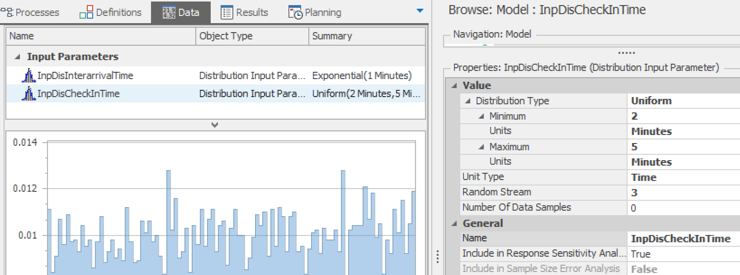
Figure 3.7: Setting Up Input Distributions
3.3.6 Now go back to your model and replace (1) the Interarrival Time in the SrcPassengersArrive to InpDisInterarrivalTime and (2) the Processing Time in the SrvCheckIn to InpDisCheckInTime. The easy way to add these input parameters is to right-click the down arrow in the specification and select the “Set Input Parameter.” From the options, select the name distributions.
3.4 Examining Output
The specific output from a simulation is a random variable produced by the entities flowing through the model and receiving services. Their arrivals and services are both random. Hence, one run/replication of the model produces one experimental value. This singular value is not precise, and to gain precision, we need to make multiple runs/replications.
3.4.1 Change the run length to 24 hours and run the simulation (i.e., use “Fast-Forward”). After the simulation is complete, click “Stop” and then click the “Results” window tab to access the results window. In the “Display” section of the SIMIO ribbon, change the units of time to minutes.
3.4.1.1 What is the average number of people waiting at check-in?
_______________________________________________
3.4.2 To gain confidence in the precision of our results, the model needs to be run for several independent replications. From the “Project Home” tab, add a new experiment to run the model multiple times by clicking on the “New Experiment” icon.
3.4.3 In the “**Design*” window tab, change the number of replications to ten20 and “Run” the experiment using the icons in the “Experiment” section of the SIMIO ribbon. It should run quickly, and the progress of each replication is shown in the comment window at the bottom. If you are running on a multi-core computer, the runs will not be in order since each replication runs on a different core.
3.4.4 You can look at the “Pivot Grid” or the “Reports” tab to get the results (remember that you can set the “units” in the ribbon for the output). From the Pivot Grid, notice that the “Results Fields” now include “Minimum,” “Maximum,” and “Half-width.” The half-width is one-half of a confidence interval with the “Confidence Level” as specified in the Experiment Properties, which is 95% by default. Recall that the confidence interval is a statement about the precision of the summary values.
3.4.5 With (1 – \(\alpha\))% as the “confidence level,” you may recall that the following formula gives the corresponding statistical confidence interval.
\[\boxed{\overline{X}\ \pm \ t_{n - 1,1 - \frac{\alpha}{2}}\frac{s}{\sqrt{n}}}\ \ \ \ \ \ \ \ \ \ \ \begin{aligned} n &= \text{number of replications} \\ \overline{X} &= \text{sample mean} \\ s &= \text{sample standard deviation} \\ t_{n - 1,1 - \frac{\alpha}{2}} &= \text{critcial value from Student t statistic} \end{aligned}\]
3.4.6 Note that:
- The statistical summary values, such as an average, are computed average values from each replication (one observation per replication). The confidence interval will increase in width as the confidence level goes from 90% to 95% to 99%, while the confidence interval gets smaller as the number of replications increases.
- The “half-width” is simply one-half the width of the confidence interval
- According to the following equation, a simulation run for n0 replications with a half-width of h0 will require (approximately) n total replications to obtain a target half-width h.
\[\boxed{n\ = n_{0} \frac{h_{0}^{2}}{h^2}}\ \ \ \ \ \ \ \ \ \ \ h_{0} = \text{half width from the observation of}\\ n_{0}\ \text{replications} \]
3.4.7 You can add the standard deviation (actually the standard deviation of the mean or standard error – not the standard deviation of bservations within a replication) by right-clicking one of the Filter Fields and selecting “Show Field List.” Next, double-click on the Std. Dev field.
3.5 Using Experiments
Suppose we want to determine the effect a change in the capacity of the check-in station will have. We could simply change the capacity and rerun the simulation, looking at the results. A better way is to set up a SIMIO “experiment” containing alternative “scenarios” that can be directly compared.
3.5.1 In the Facility view, click on the SrvCheckIn object. Right-click on the Initial Capacity property and select “Set Referenced Property.” Use”Create New Property” and give it the name CheckInCapacity. Doing this creates a new model “property,” which is listed in the “Definitions” tab of the model under the “Properties” listing.
3.5.3 Add Scenario rows, changing the CheckInCapacity to two, three, and four to create an experiment grid, as seen in Figure 3.8. You can add rows by clicking on the “*” symbol in the first column. Essentially, you are defining three scenarios, each having a different check-in capacity.
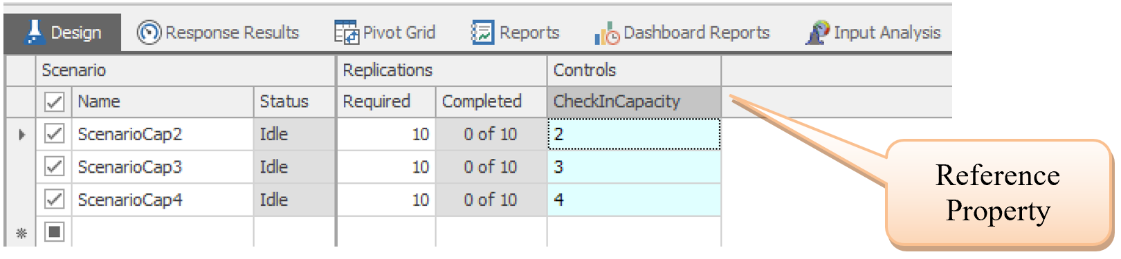
Figure 3.8: Experiment Scenarios
3.5.4 Now run the simulation, performing ten replications of each scenario, which is completed very quickly.21 SIMIO will parallel process the experiments on each core of a multi-core computer. Replications that finish turn green in parallel with the yellow scenarios that are currently being run.
3.5.6 The “Reports” tab is an excellent way to compare scenarios. In the reports tab, the scenarios are organized under each data item.
3.5.7 It is helpful to add “responses” to the experiment to aid in comparing scenarios. Simply click the “Add Response” button in the “Design” tab. Insert the following two responses with expressions that will look at the average time in the system by the passengers and the total number processed, specifying units of minutes for the time in the system, as seen in Figure 3.9.
- TimeInSystem, in Minutes: EntPassenger.Population.TimeInSystem.Average
- TotalNumberProcessed: EntPassenger.Population.NumberDestroyed
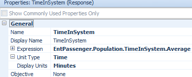
Figure 3.9: Specifying the Time in System
3.5.8 Reset and rerun the experiment, looking at the “Response Result” charts and the scenario grid (see Figure 3.10). To arrange the “tabs,” click a tab and drag it to the desired position on the display—note the positioning points. You can also right-click a tab to configure the display of results.
3.5.9 The Response Results and the SMORE22 plots contain graphical displays of various summary results from each scenario. Generally, the numerical values are hard to determine from just the graph, which will be discussed later. Still, the graph helps to show trends and variations across and within scenarios. The confidence interval on the mean, which is most often used, is displayed in the rust color. If confidence intervals between scenarios don’t overlap, the senarios are statistically different.
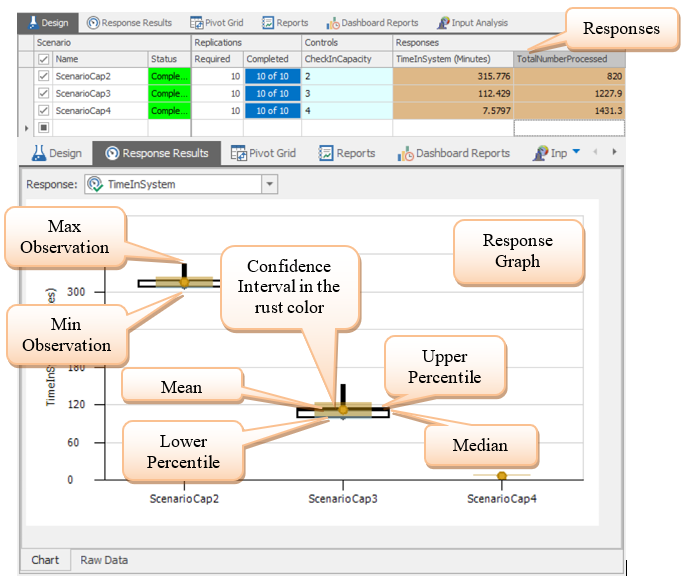
Figure 3.10: Response Results
3.5.11 If you select the “Raw Data tab found at the bottom of the “Response Results” tab, you will get the table shown in Figure 3.11, which includes numerical details on the responses, the confidence interval (95%) on the response, and the percentiles (which are 25% and 75% by default).23
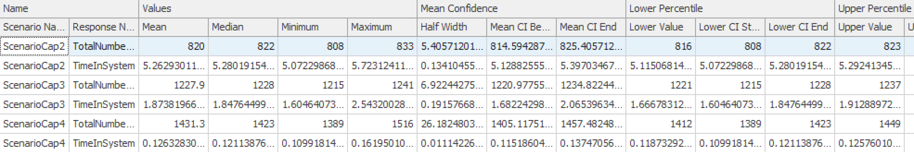
Figure 3.11: Raw Data on Graph
3.6 Input Sensitivity
Since we specified the interarrival time and processing time as “input parameters” and our experiment has responses with multiple replications greater than the number of input parameters, SIMIO can perform a sensitivity analysis on these inputs as a by-product. Essentially, this analysis attempts to determine how the inputs affect the responses (i.e., outputs) through simple linear regression.
3.6.1 Click on the “Input Analysis” window tab for the experiment and select the “Response Sensitivity” panel icon. Select, for example, “ScenarioCap2” and the “TimeInSystem” response.
3.6.2 Four lower tabbed displays (i.e., Tornado Chart, Bar Chart, Pie Chart, and Raw Data) are available. Each chart measures how the particular “input” affects the particular “response” relative to each other. The numerical values associated with the graph are displayed by moving the mouse over the display. The Tornado chart shows a single response, whereas the bar and pie charts show all responses together, as seen in Figure 3.12.
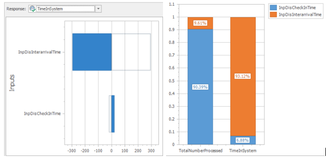
Figure 3.12: Tornado Chart for Sensitivity of Input to Time in System
3.6.4 Step 4: In the tornado chart, the solid line shows the relation between the input parameter and the response, while the outlined bar shows the negative. In this case, the lower the interarrival time (i.e., faster arrivals), the higher the time in the system. Meanwhile, the higher the processing time, the higher the time in the system. Clearly, from the figure, the interarrival time has a much more significant influence on time in the system than the processing time. However, from the bar chart, the reverse is true for the total number processed. This information can help modelers determine if more data needs to be collected to verify the input distribution assumptions.
3.6.5 Although the impact of adding capacity to the check-in is evident in Figure 3.6, the capacity can be considered an input parameter and added to the sensitivity displays.
3.7 Commentary
- Once you have a working model, you need to verify and validate your model. Is our model free of modeling and programming errors and working as intended (i.e., verify our model)? Does our model represent what is happening in the real world relatively well (i.e., validate the model)? We can never model exactly what is happening in the real world, but can we capture enough of the essence of the actual system to make a decision? For example, one can compare the actual values of a response to the confidence intervals created from the simulation experiment.
- The standard deviation produced in the output (see the “Results Field” option) is really the standard error (standard deviation of the mean). No standard deviation is computed within one run of the simulation, even though it can be computed and can provide some helpful modeling options (for instance, in establishing inventory policies). The danger is that the standard deviation calculated within a single replication cannot be used to compute a legitimate confidence interval since the observations may not be Normally distributed nor independent and identically distributed (IID).
- The sensitivity of input parameters on individual responses opens up a helpful method to explore the behavior of the simulation model, as seen in later chapters.
- Later chapters will describe the SMORE plots, subset selection, ranking/selection, and optimization in detail.
- While other simulation languages may manage the output in a database file, SIMIO manages the output internally, but it can be exported externally.
To connect objects via links without selecting them from the [Standard Library], hold the Ctrl Shift keys down while selecting the TransferNode to start the drawing of the link. After completing the link, choose the correct link.↩︎
You can also add more than one symbol for the passenger as was done in Chapter 2.↩︎
New symbols can be created by packages like Trimble’s SketchUp Pro™ as well as other 3-D graphics software.↩︎
Distribution allows one to specify a single distribution which can be used in both sensitivity and sample size error analysis by specifying the number of samples used to build the distribution.↩︎
A random number stream for a distribution can be viewed as a specific series of random observations from that distribution. As such, it is reproduced by choosing that same stream again. This insures that the randomness associated with that stream is reproduced in other scenarios, so its randomness doesn’t add additional variance to the output performance measures.↩︎
It should have defaulted to ten.↩︎
Run the experiments under the “Design” tab in the SIMIO ribbon to employ the scenario controls. If you go back to the Facility window to run the simulation, then the controls employ their original specifications.↩︎
SMORE is SIMIO Measure of Risk & Error↩︎
You can change the confidence level and percentiles in the Experiment properties.↩︎