Simulation Modeling with Simio - 6th Edition
Chapter
1
Introduction to Simulation: The Ice Cream Store
This chapter will give the novice in simulation an introduction to the terminology and mechanics of simulation, as well as statistics and performing a simulation model. If you are already familiar with these concepts, feel free to start with Chapter 2, which starts the simulation modeling in SIMIO™.
1.1 What is Simulation?
The word “simulation” has a variety of meanings and uses. Probably its most popular usage is in games. A video game “simulates” a particular environment, maybe a Formula One race, a battle, or a space encounter. The game allows the user to experience something similar to driving in a race, maybe with other people participating. In the military, commanders create a battlefield simulation where soldiers act according to their training, perhaps by defending a base or assaulting an enemy position. In aeronautical engineering, an engineer may take a model airplane to a wind tunnel and test its aerodynamics. Most simulations have elements of reality with the intention that the participant will learn something about the environment through the simulation or perhaps only learn to play the game better.
We employ simulation to study and improve “systems” of people, equipment, materials, and procedures. We use simulation to mimic or imitate the behavior of systems like factories, warehouses, hospitals, banks, supermarkets, theme parks – just about anywhere a service is provided or an item is being produced. Our simulations are different from gaming and training simulations in that we want the simulation to model the real system so we can investigate various changes before making recommendations. In that sense, simulation is a performance improvement tool. The simulation acts as an experimental laboratory, except that our laboratory is not physical but instead a computer model. We can then perform experiments on our computer model.
Modeling
Many performance improvement tools (e.g., Lean, Six Sigma, etc.) rely on models. For example, value stream maps, spaghetti diagrams, process flow charts, waste walks, etc., are helpful conceptual/descriptive models for performance improvement based on direct observations of the system. These models provide a wide range of vehicles for describing and analyzing various systems. More formal models employ mathematical and statistical methods. For example, linear regression is a popular modeling technique in statistics. Queuing models offer a means for describing an important group of stable stochastic processes. Linear programming is a formal optimization method of finding the values of variables that minimize or maximize a linear objective function subject to linear constraints. Nevertheless, all these methods require various assumptions about the system being modeled. For example, the variables are constants (i.e., real or integer-valued) and often related linearly. If the variables have statistical variation, they are assumed to be normally or exponentially (i.e., Markovian) distributed.
Simulation is a model-based improvement tool. However, a few assumptions need to be made to build the model. The model can be non-linear, described by arbitrary random variables, have a complex relationship, and change with time (i.e., dynamic). In fact, the simulation model is limited only by your imagination and the nature of the system being considered. You determine the nature of the model based on what you think is important about the system being studied.
Computer Simulation Modeling
Instead of a formal model, our simulations are computational. The model is essentially a logical description of how the components of a system interact. This description is translated into a computational structure within the computer using a simulation language. The computer simulation of the system is executed over and over to generate statistical information about the system’s behavior. We use statistics to describe the system’s performance measures. We modify the computer simulation models to study alternative systems (i.e., experiments) based on what we learn about the system. By comparing these alternative systems statistically, we can offer performance improvement recommendations.
Of course, we could experiment directly with the system. If we thought an additional person on the assembly line would improve its production, we could try that. If we thought a new configuration of the hospital emergency room would provide more efficient care, we could create that configuration. If we thought a new inventory policy would reduce inventory, we could implement it. But now, the value of a computer simulation model becomes apparent. A change in a computer simulation model is cheaper and less risky than changing the real system. Using a computer simulation to determine if the changes are beneficial is also faster. Also, it might be safer to try a change in a simulation model than to try it in real life. In general, it is much easier to try changes in a computer model than in a real operating system, especially since changes disrupt people and facilities.
A computer simulation model allows us to develop confidence in making performance improvement recommendations. We can try out various alternatives before disrupting an existing system. You can now see why many companies and managers require that a simulation study be done before making substantial changes to any working system, especially when there are potential negative consequences of performance changes and costs that don’t provide improvement.
Verification and Validation
Since simulation models often have serious consequences and are developed with a minimum set of assumptions, their validity must be carefully considered before we believe in the recommended benefits. In simulation, we often use the words “verification” and “validation,” and we have specific definitions for each.
The word “verification” refers to the model and its behavior. We most often develop our simulation models with a simulation language. This language translates our modeling “intent” into a computation structure that produces statistics. Most simulation languages can be used to describe a complex operating system, and the language provides a framework of components for viewing that system. As our models become more complicated, we employ more complex simulation language constructs to model the behavior. This relationship is critically dependent on our understanding of the simulation language intricacies. We may or may not fully understand the computational code, and thus, we confront the key question in verification: Does the simulation model behave the way we expect? Could we have made a mistake in employing the simulation language, or does the simulation language create an unexpected behavior in the computational code? Therefore, even after we have created our simulation model, it needs to be tested to see if it behaves as expected. If we make the processing time longer, does it result in longer times in the system? Does the waiting time decrease if we reduce the arrival rate to a queue? The answers to any of these questions are specific to the system and your model of it. But, above all else, we need to be sure that our model is behaving the way we expect without error.
The word “validation” refers to the relationship between the model and the real system (i.e., Does the simulation produce performance measures consistent with the real system). Now, we are assuming our model has been verified, but can we validly infer from the real system? This question strikes at the heart of our modeling effort because we cannot legitimately say much about performance improvement without a valid model. Many people new to simulation may want the model to be a substitute for the “real system,” which is a limitless task. After all, the only “model” that is perfectly representative of the real system is the system itself!
We must always remember in simulation that our model is only an approximation of the real system. So, the most relevant way to validate our model is to concern ourselves with its approximation. How do we decide what to approximate? It depends on our performance measures. If our performance measure is time in the system, then we concern ourselves with those factors that impact time in the system. If our performance measure is production, then we focus on those factors that impact production. Usually, we are interested in several performance measures, but those measures will be the focus of our concern and will limit our modeling activity. Otherwise, without a clear set of performance objectives, we are left with a search for reality in our model, which is a never-ending task.
Generally, people who are only familiar with simulation think simulation models can mimic anything and often drive the development of a needlessly complex model. One of the difficult responsibilities of anyone engaged in simulation modeling is to educate the stakeholders on the benefits and limitations of a simulation model as well as the simulation modeling activity.
Computer Simulation Languages
The process of creating a computer simulation model varies from programming your own model in a programming language such as C++, C#, Python, or Java to using a spreadsheet like Excel. There are a variety of simulation languages including Simula™, GPSS™, SIMSCRIPT™, Arena/SIMAN™, SLX™, ProModel™, Flexsim™, AutoMod™, ExtendSim™, Witness™, AnyLogic™, among many others. Each simulation language differs in how it requires users to construct a simulation model. An important distinction is the degree to which computer programming is required. Also, many of the simulation languages have evolved from a particular industry or set of applications and are especially useful in that context.
We have chosen to use the simulation language SIMIO™, a relatively new language developed over the past several years. The language developers had previously developed the Arena simulation system. SIMIO benefits from more recent developments in object-oriented design and agent modeling. SIMIO is a “multi-modeling” language with agents, discrete event, and continuous language components. SIMIO was developed to provide visual appeal through its 3-D animation and graphical representations. SIMIO provides a wide range of extensions, from direct modification of executing processes to user-developed objects. SIMIO also provides interoperation with various spreadsheets and databases. Finally, SIMIO has become widely adopted in industry and academic institutions. Learning SIMIO provides one broadly-based simulation modeling tool that can help you learn to use others if needed.
1.2 Simulation Fundamentals: The Ice Cream Store
A fundamental understanding of simulation will be beneficial throughout your study of simulation. It’s easy to get caught up in the creation of a computer model using a simulation language and miss important basic principles of simulation modeling. Too many people associate simulation with a simulation language; for them, simulation is simply learning the language. Learning a simulation language is necessary for using simulation, but it does not substitute for understanding at a fundamental level. If you understand the fundamentals of simulation, you establish a basis for understanding any simulation language and model. In fact, this understanding will be a key to learning almost everything else in this text.
The Ice Cream Store
It is helpful if the discussion of simulation is done in the context of a problem – albeit a simple problem. Using this simple problem, we can describe simulation elements of modeling, execution, and analysis. Our problem is the common ice cream store since everyone loves ice cream and probably has visited an ice cream store. As seen in Figure 1.1, customers arrive at the ice cream store to obtain an ice cream cone. It’s a simple store where there is only one attendant, and people will wait in a single line to order and receive their ice cream cone. The attendant waits on each customer, one at a time, in the order they arrive.
1.2.0.1 What might be your operational concerns if you owned or managed the ice cream store?
_______________________________________________
Likely, one of your most prominent concerns would be this store’s operation and how you can improve it. For example, could you buy a new cone-making machine to make cones faster, or should you hire someone to help service customers? Should you resize the waiting space? These are performance improvement concerns.
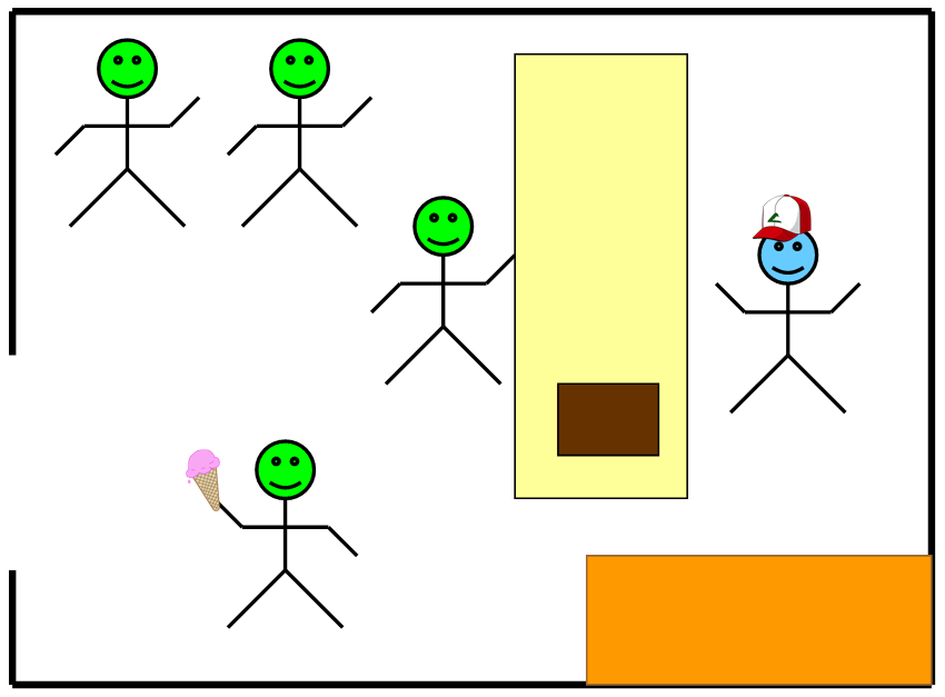
Figure 1.1: The Ice Cream Store
1.2.0.2 If you made one of these changes to the ice cream store, how would you decide if it improved the store’s operation?
_______________________________________________
In other words, what are the performance measures? Here are some possible measures: the number of customers served per day, the time customers spend in the store, the waiting time of customers, the number of customers waiting, and the utilization of servers. We will discover these are common performance measures and will often be your first performance measurement choices.
1.2.0.3 How can you expect to improve performance if you don’t know what is happening inside the ice cream store?
_______________________________________________
You need to employ all the descriptive tools you know to understand what is going on inside the system. At this stage, one might create a value stream map, a flow chart, a relationship chart, a spaghetti diagram, etc. These techniques will greatly improve your understanding of what happens to customers and the attendants during the sale of an ice cream cone. Perhaps you develop the conceptual model (i.e., flow chart) presented in Figure 1.2.
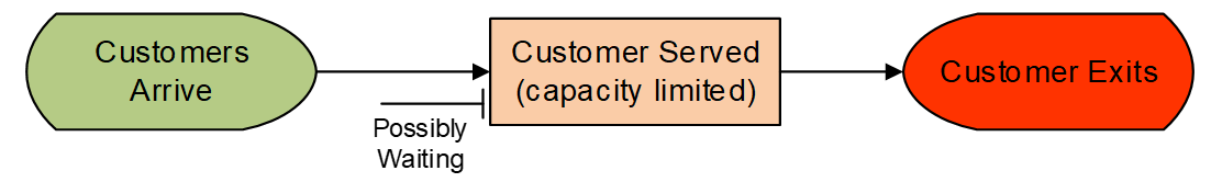
Figure 1.2: Flow Chart of the Ice Cream Store
The conceptual model shows how the customers are served. Notice that we have added the possibility of waiting due to the fact that the availability of a single attendant limits service.
Gathering Data about the Ice Cream Store
Descriptive information helps us understand the service process in the ice cream store; however, it doesn’t give us the performance measures. For that, we need to document what is happening (i.e., we need to do a “present systems analysis”). Suppose we decide to do a “time study” of the store operations, as shown in Table 1.1.
| Time | Customer | Process |
|---|---|---|
| 0.00 | Store Opens – Server Idle | |
| 0.00 | 1 | Arrives |
| Start service on Customer 1 – Server Busy | ||
| 8.36 | 1 | Departs service – Server Idle |
| 9.01 | 2 | Arrives |
| Start service on Customer 2 – Server Busy | ||
| 9.98 | 3 | Arrives – Customer 3 waits |
| 13.5 | 4 | Arrives – Customer 4 waits |
| 19.36 | 2 | Departs Service – Customer 2 leaves: |
| 3 | Start service on Customer 3 – Server Busy | |
| 23.07 | 5 | Arrives – Customer 5 waits |
| 27.22 | 3 | Departs service – Customer 3 leaves: |
| 4 | Start service on Customer 4 – Server Busy | |
| 33.82 | 4 | Departs service – Customer 4 leaves: |
| 5 | Start service on Customer 5 – Server Busy | |
| 38.18 | 6 | Arrives – Customer 6 waits |
| 40.0 | End observations |
In our time study, we simply record all the “events” and the event time that occurs in the ice cream store. An event occurs when something operationally happens in the store, like an arrival of a customer or the departure of a customer from service. Also, we recorded when the attendant (i.e., server) becomes busy or idle. Here, we only observed the first 40 minutes of the store’s operation. We recognize this isn’t enough time to gain a full understanding, but we do not intend to solve a problem at this time – only to demonstrate a method.
The time study is sufficient for us to compute some performance measures, but first, it will be helpful to re-organize our time study data. We are not going to add (or subtract) any information. We are simply going to re-organize our data from an event view to an entity (i.e., customer) view. The event view records events, but the entity view allows us to follow our customers. The re-organized data is shown in Table 1.2, which shows when the customer arrives at the store, enters service, and leaves the store. Notice that customers five and six service and exit the store after 40 minutes.
| Customer | Arrives to Store | Enters Service | Leaves Store |
|---|---|---|---|
| 1 | 0.00 | 0.00 | 8.36 |
| 2 | 9.01 | 9.01 | 19.36 |
| 3 | 9.98 | 19.36 | 27.22 |
| 4 | 13.5 | 27.22 | 33.82 |
| 5 | 23.07 | 33.82 | ?? |
| 6 | 38.18 | ?? | ?? |
Performance Measure Calculations
From the entity view of the time study data, we can easily compute several performance measures.
- Production: Number of people served. The number of people served is easily calculated by looking at the number of customers that have exited the system in the simulation time. In our example, four people were served in 40 minutes, or the system had a production rate of six per hour (i.e., four customers/40 minutes * 60 minutes/hour).
- Flowtime, Cycle Time: Time in System. The time in the system is calculated by averaging the difference between when the customer entered and exited the system. Again, only four customers exited the system and contributed to the average time in the system in our simple ice cream system, as seen in Table 1.3.
| Customer 1 | Customer 2 | Customer 3 | Customer 4 | Average Time in System |
|---|---|---|---|---|
| 8.36-0.0 | 19.36-9.01 | 27.22-9.98 | 33.82-13.5 | 56.27/4 = 14.07 minutes |
- Non-Value Added Time: Waiting Time in Queue. The time in queue (i.e., the waiting or holding time) represents the time customers waited in line before being seen by the ice cream attendant. It is calculated by averaging the difference between when the customer entered the system and when they entered the service. During our observation window, five customers entered service, as seen in Table 1.4.
| Customer 1 | Customer 2 | Customer 3 | Customer 4 | Customer 5 | Average Waiting Time |
|---|---|---|---|---|---|
| 0.0-0.0 | 9.01-9.01 | 19.36-9.98 | 27.22-13.50 | 33.82-23.07 | 33.85/5 = 6.77 minutes |
- Number Waiting In Queue: This measure determines the average number of customers one would expect to see waiting in line to receive service. Unlike the previous metrics, the number waiting in queue or number in the system measures are time-persistent or time-weighted statistics. You may have never computed a time-persistent statistic, which is a statistic for which we need to know the amount of time a value was observed. The value of the observation is weighted by the amount of time that value persists. A graphical depiction of the number in the queue at the ice cream store is in Figure 1.3.
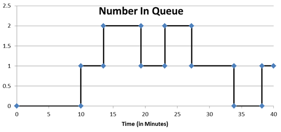
Figure 1.3: Graph of the Number in Queue in the Ice Cream Store
Consider computing the average number in the queue. Suppose we observed the number in the queue to be two one time and ten another time. Would you say that on an average number, we would expect to see six in line? Of course “not”! You need to know how long the value of two was observed and how long the value of ten was observed. Suppose we observe two in the queue for ten minutes of the time and ten in the queue for only one minute. So the queue was observed for a total of 11 minutes. As a result, the value of two was observed 10/11ths of the total time while ten was observed 1/11th of the total time. Our average then is 2*(10/11) + 10*(1/11) or = 2.73 customers. Another way of computing is to realize that the total waiting time1 observed was 20 + 10 over a total of 11 minutes, which also yielded 2.73 people. Now, looking at the data from the ice cream store, we need the percentage of time (40 minutes) that there was zero waiting, one waiting, two waiting, three, and so forth2. In our case, a maximum of two was observed, and the waiting time would be computed as seen in Table 1.5.
| Number In Queue | Time Period | Time Spent (min) |
|---|---|---|
| 0 | 0.00 – 9.98 | 0*9.98 = 0.000 |
| 1 | 9.98 – 13.5 | 1*3.52 = 3.520 |
| 2 | 13.50 – 19.36 | 2*5.86 = 11.72 |
| 1 | 19.36 – 23.07 | 1*3.71 = 3.710 |
| 2 | 23.07 – 27.22 | 2*4.15 = 8.300 |
| 1 | 27.22 – 33.82 | 1*6.60 = 6.600 |
| 0 | 33.82 – 38.18 | 0*4.36 = 0.000 |
| 1 | 38.18 – 40.00 | 1*1.82 = 1.820 |
| Total Waiting Time | 35.67 minutes | |
| Average Number in Queue | 35.67/40 = 0.89 Customers |
- Utilization: This performance is the percentage of time the server is busy servicing customers, which is calculated by dividing the time spent servicing customers by the total time available. For our example, the attendant is only idle during the time period between finishing servicing customer one and the arrival of customer two (i.e., 9.01 – 8.36 = .65 minutes). Therefore, the attendant’s utilization will be 39.35/40 or 98.4%:
- Other possible performance measures are maximum values, standard deviations, time between departures, etc.
There are three main types of simulation performance measures, counts, observation-based statistics, and time-persistent statistics, as described in Table 1.6.
| Type | Description/Examples |
|---|---|
| Counts | The number of parts that exited, entered, etc. (e.g., production). |
| Observation-based Statistics | These measures typically deal with time, such as waiting time, time in the system, etc. SIMIO calls observation-based statistics “Tally” statistics. |
| Time-Persistent/Time-Average Statistics | These measures deal with numbers in the system, queue, etc., when the values can be classified into different states. SIMIO calls these “State” statistics. |
1.2.0.4 What is another example of an observations-based performance measure?
_______________________________________________
1.2.0.5 What is another example of a time-persistence performance measure?
_______________________________________________
1.2.0.6 Is average “inventory” a time-persistent or observation-based statistic?
_______________________________________________
1.2.0.7 Is the amount of time that a job is late a time-persistent or observation-based statistic?
_______________________________________________
Terminology of a Queuing System
Figure 1.4 shows some elements of a “common” queueing system with the normal terminology. We will generally refer to the arriving objects as “model entities” and the counter/attendant as a “server.” You can see the members of the queue and the customer in service. The input processes for this system are the arrival process and service processes. We will provide details on these inputs later.
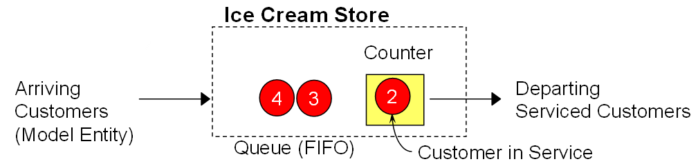
Figure 1.4: A Breakdown of Terminology
Can We Simulate It?
We want to reproduce the time-study data collection exercise we used for the ice cream store. But we want to synthesize it numerically as opposed to observing it – in essence, simulate it! We can compute the performance measures if we can recreate the time study data. Notice that the time study records are centered on “events.” Recall these events are points in time when the system changes its state (i.e., status). A quick review of that data reveals that three types of events occur, as described in Table 1.7.
| Number | Type | Event Description |
|---|---|---|
| 1 | Arrival | Indicates an entity will arrive at this time. |
| 2 | End of Service | An entity will be departing from service (i.e., service has finished) |
| 3 | End | The simulation will terminate and end all observations. |
We need a method to keep track of our events to facilitate our simulation. Although there are other ways to keep track of events, keeping them in an “event calendar” is convenient. An event calendar contains the records of future events (i.e., things we think are going to happen in the future), ordered by time (with the earliest event first). Simulation can be executed by removing and inserting events into the event calendar.
Let’s add some specifics to our simulation problem (i.e., the ice cream store). We will use “minutes” as our base measure of time. The input data that we currently have is shown in Table 1.8.
| Customer | Arrival Time | Interarrival Time | Processing Time |
|---|---|---|---|
| 1 | 0.00 | 0.00 | 8.36 |
| 2 | 9.01 | 9.01 | 10.35 |
| 3 | 9.98 | 0.97 | 7.86 |
| 4 | 13.50 | 3.52 | 6.60 |
| 5 | 23.07 | 9.57 | 8.63 |
| 6 | 38.18 | 15.11 | 10.33 |
| 7 | 42.08 | 3.90 | 10.46 |
| 8 | 48.80 | 6.72 | 7.96 |
In Table 1.8, the arrival time has been re-stated as an “interarrival time” – namely time between arrivals. This re-statement does not change the arrival times but simply how they are presented. Such a representation also requires the time of the first arrival from which the interarrival times are sequentially computed. Table 1.8 provides data on only the first customers. We may need more data, but this will be discussed later.
The Simulation Algorithm
To synthesize the system as presented in the time study, we need a systematic means of moving through time by removing and inserting events on the event calendar. Consider the simulation algorithm shown in Figure 1.5.
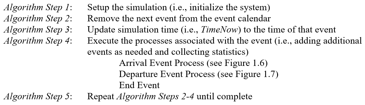
Figure 1.5: Simple Simulation Algorithm
Remember that the event calendar is ordered according to the next most recent event. So, we can move through time by removing the “next” event from the event calendar, updating time to the time of that event, and executing whatever processes are associated with that event. This simple method is then repeated until we reach some terminating time or condition.3 In our case, the “events” are the arrival of an entity, the service (departure) of the entity, and the end of the simulation period. The arrival and departure of the entities are the most important. Consider now how the arrival (see Figure 1.6) and the departure (see Figure 1.7) are processed within the context of our simple single queue, single server system. The word “schedule” means to insert this event into the event calendar.
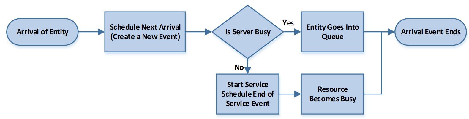
Figure 1.6: Event Process Associated with Arrival of Entity
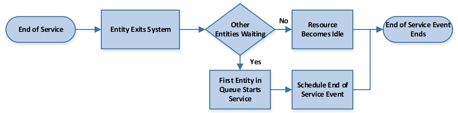
Figure 1.7: Event Process Associated with End of Service
The arrival of an entity creates a new event because we know the next entity’s arrival time since we have the interarrival times of entities. The newly arriving entity either must wait because the server (i.e., resource) is busy, or that entity can engage the server and start service. If the entity can start service, we now know a new future event, namely the service departure, because we know the processing time. So, suppose the removed event is an arrival. In that case, we insert the next arrival into the event calendar and may insert the service departure event in the event calendar, provided the entity can start service immediately. If the event removed from the event calendar is a service departure, then the entity that has finished service will exit the system. If the waiting queue is empty, then the resource (server) becomes idle. On the other hand, if at least one customer is in the queue, the first customer is brought into service, the resource remains busy, and a new future event, namely the service departure, is inserted into the event calendar because we have the processing time. Note that a service departure causes the entity to depart the system regardless of what happens to the server.
1.2.0.8 What is the maximum number of new events that are added to the event calendar when an entity arrival event occurs? What are they?
_______________________________________________
1.2.0.9 What is the minimum number of new events that are added to the event calendar when an entity arrival event occurs?
_______________________________________________
1.2.0.10 What is the maximum number of new events that are added to the event calendar when an entity departure event occurs? What are they?
_______________________________________________
1.2.0.11 What is the minimum number of new events that are added to the event calendar when an entity departure event occurs?
_______________________________________________
Finally, we note that the very first step of the simulation algorithm calls for the system to be “initialized.” In other words, how will we start the operation relative to the number of entities in line and the state of the server? It will be convenient to use the “empty and idle” configuration. By “empty and idle,” we mean that the server is idle and the system is empty of all entities.
1.3 Manual Simulation
A simple data structure will be employed to execute a manual simulation, as seen in Figure 1.8, to further understand how a discrete event simulation operates. Our manual simulation will consist of a “system animation” graphical representation of what is going on in the system, with the current customer being serviced shown inside the square and other customers waiting outside the square. The current simulation time (i.e., called “Time Now”) will be shown. The current event will be identified, followed by a description of the process. Finally, the “Event Calendar” will be maintained, which will include the event time, event type, and entity ID number.
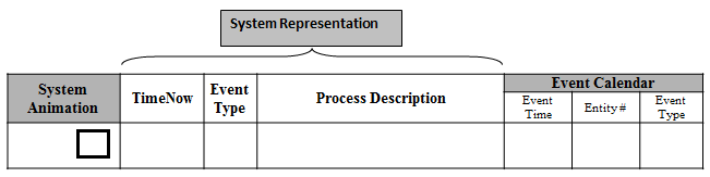
Figure 1.8: Manual Simulation Data Structure
1.3.1 Algorithm Step 1 of the simulation, as defined in Figure 1.5, is used to “initialize” the system as seen in the executing structure of Figure 1.9. Note that we have inserted the time of the first entity arrival into the event calendar, and we have inserted the end event or the time to stop making observations.
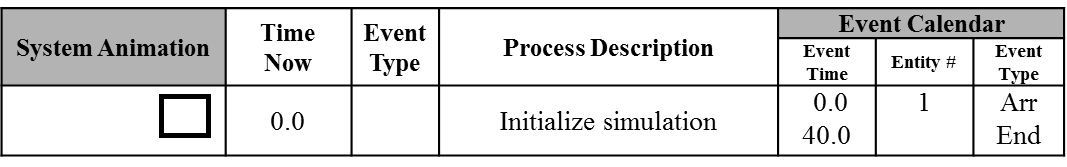
Figure 1.9: System Initialization
1.3.2 Executing the simulation algorithm, we remove the next event (Algorithm Step 2) from the event calendar, update the simulation time to the time of that event (Algorithm Step 3), and execute the appropriate processes (Algorithm Step 4). The next event is the “Arrival of Entity #1” at time 0.0. The arrival of this entity allows us to schedule into the Event Calendar the “Arrival of Entity #2” to occur since the interarrival time between Entity #1 and Entity #2 is 9.01 minutes, and thus the Arrival event for Entity #2 is at time 9.01 (i.e., 0.0 + 9.01). Because Entity #1 arrives when the server is idle, that entity enters service, and we can now schedule its Departure event because we know the processing time for Entity #1 as 8.36 minutes; thus, the event time is 8.36 (i.e., 0.0 + 8.36). The result is that our data structure now appears in Figure 1.10.
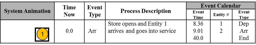
Figure 1.10: Processing Time 0.0 Event
1.3.3 We are done with the processes associated with time 0.0. The next event in the event calendar is the “Departure of Entity #1” from the system at time 8.36. Since there are no entities in the queue, the server is allowed to become idle, and no new events are added to the event calendar, as shown in Figure 1.11.
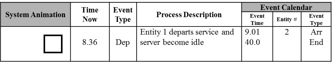
Figure 1.11: At Time 8.36
1.3.4 The next event is the arrival of Entity #2 at time 9.01. So, we remove it from the event calendar and update the simulation time to 9.01. We can schedule the arrival of Entity #3 at the current time (9.01) plus the interarrival time from Entity #2 to Entity #3 (0.97), which is event time 9.98. Next, Entity #2 can start service immediately since the server is idle, so its departure event can be scheduled as the current time (9.01) plus the processing time for Entity #2 of (10.35), which yields an event time of 19.36. The new status of the simulation is shown in Figure 1.12. We have also added an animation showing the status of the entities and the server.
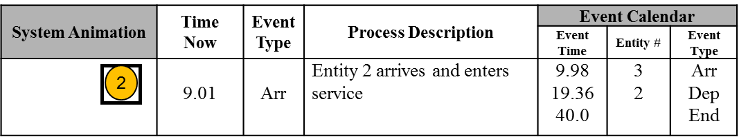
Figure 1.12: At Time 9.01
1.3.5 The next event occurs at time 9.98, which is the arrival of Entity #3. Its arrival allows us to schedule the next arrival (i.e., Entity #4) at time 13.50. But now the arriving entity must wait, as indicated in the “System Animation” section of the data structure in Figure 1.13.
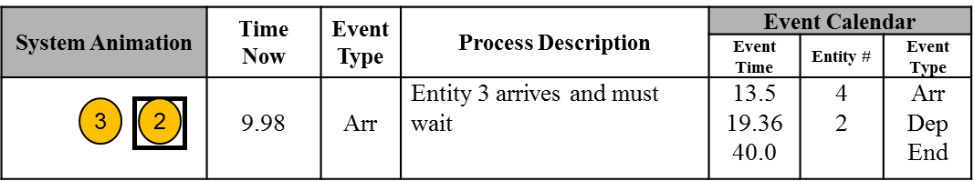
Figure 1.13: At Time 9.98
1.3.6 The next event is the arrival of Entity #4, which will schedule the arrival of Entity #5 but will have no other actions since the server remains busy. The new simulation time is 13.50, and the updated status is shown in Figure 1.14
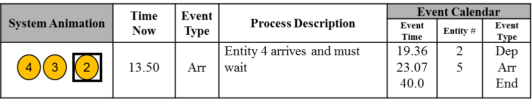
Figure 1.14: At time 13.50
1.3.7 Finally, we see that Entity #2 finishes service at 19.36 and departs. Entity #3 can go into service, and we can schedule the service departure of Entity #3 at 27.22, as shown in Figure 1.15

Figure 1.15: At Time 19.36
1.3.8 From Figure 1.15, we see the next event, which is the arrival of Entity #5 at time 23.07, which triggers the addition of the next arrival (Entity #6), as shown in Figure 1.16.
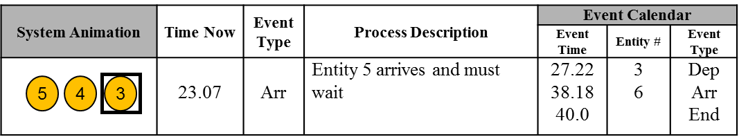
Figure 1.16: At Time 23.07
1.3.9 Entity #3 completes service at 27.22, allowing Entity #4 to enter serviced, which schedules the end-of-service event for Entity #4 at 33.82, as shown in Figure 1.17.
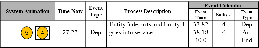
Figure 1.17: At Time 27.22
1.3.10 The result of this next event is shown in Figure 1.18.
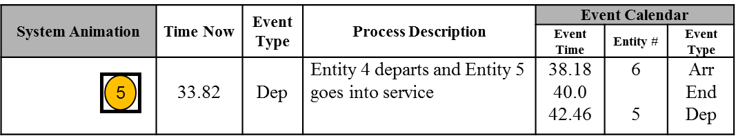
Figure 1.18: At Time 33.82
1.3.11 We are getting closer to the time to quit observing the system; however, we have one more event and one more time update. The result of this next event is shown in Figure 1.19.
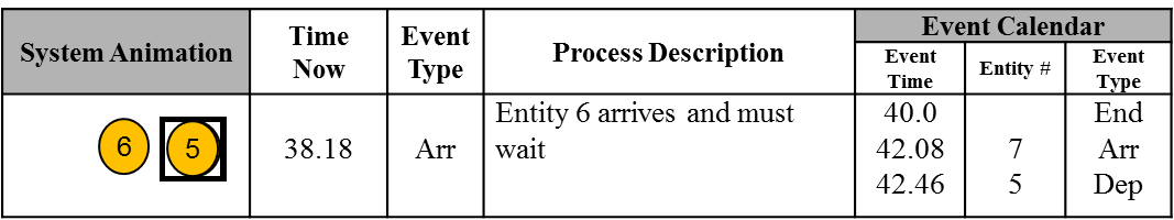
Figure 1.19: At Time 38.18
1.3.12 Finally, the next event calls for the “End” of the simulation at time 40.0. Only time is updated as the event calendar is unchanged. The final state is given in Figure 1.20.

Figure 1.20: At Time 40.0
Our simulation approach is referred to as a “Discrete-Event Simulation” because the system only changes states at defined event times, and the state changes are discrete in that the number in the queue changes discretely, as well as the number in the system. If our model included variables that changed continuously with time, like the water in a tank, then we wouldn’t have a discrete-change system and would have to consider all points in time, not just those when the system changes state. Simulations that contain continuous variables are called “Continuous Simulations.” We can also have combinations of the two types of simulations. In fact, SIMIO can model both kinds of systems together – a multi-method simulation language.
1.4 Input Modeling and Simulation Output Analysis
Since we have now simulated the ice cream store time study, we can re-organize this information from an entity viewpoint and compute the same performance statistics that we computed previously!
1.4.0.1 Do we have enough information to draw conclusions about the present system?
_______________________________________________
1.4.0.2 What can we do to extend the information available?
_______________________________________________
If we had a total of 45 interarrival times and 43 processing times, we could simulate a total of 480 minutes of time. For example, we may obtain the information given in Table 1.9. We have included the minimum, maximum, and average values over the 480 minutes. Currently, we are simulating “only” one day for 480 minutes.
1.4.0.3 Now, do you have enough information for a “present systems analysis?
_______________________________________________
1.4.0.4 Is a one-day simulation long enough?
_______________________________________________
| Performance Measure | Value |
|---|---|
| Total Production | 43 customers |
| Average waiting time in queue | 9.59 minutes |
| Maximum waiting time in queue | 35.65 minutes |
| Average total time in system | 17.87 minutes |
| Maximum total time in system | 42.65 minutes |
| Minimum total time in system | 7.46 minutes |
| Average number of customers in queue | 0.88 customers |
| Maximum number of customers in queue | 4 customers |
| Ice Cream Attendant utilization | 78% |
One day doesn’t give us much information about the day, so more “days” of information are needed. But that means more interarrival times and more processing times. If we did a simulation of ten days, we would need approximately 450 interarrival times and 430 processing times. If that information came from an electronic record, then getting more data may not be a problem.4 However, if our only alternative is time studies, we will need to observe for ten days, which may be a greater intrusion into the actual operation than we expect.
An alternative to more data collection is for us to find a “model” of this input data (i.e., interarrival and processing times). Perhaps we can use a statistical representation since processing times and interarrival times are most certainly random variables. We can often match the processing times and interarrival times to standard statistical distributions. First, we make a histogram of the data we observed. Second, to match the data, we try to pick out a statistical distribution, like a Gamma, Lognormal, Weibull, or Pert. In fact, a wide range of software can help with this undertaking. An example of this activity is shown in Figure 1.21.
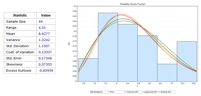
Figure 1.21: Matching Observed Processing Time to a Standard Statistical Distribution
As a result of this input modeling, we can characterize a random processing or interarrival time by a statistical model (i.e., distribution). For example, we might use a Pert distribution which has three parameters: Pert (6, 8, 12) for a processing time or maybe a Gamma distribution which has two parameters: 6.3 + Gamma(3.1, 0.7) where the 6.3 is the “location” of the distribution’s origin.
Once we characterize an input with a statistical model, simulation technology allows us to “sample” from that statistical model. Repeated sampling will statistically reproduce the input model but, more importantly, give us an “infinite” supply of input data. With that extended data, we can simulate many days of operation. Having many days of simulation allows us to gain an estimate of the precision of the average performance measures we compute. For example, suppose we simulate our system for five days. Using simulation terminology, we performed five “replications” or “runs” of our simulation model. Each replication obtains new “samples” for its interarrival times and processing times. To compute the average and the standard deviation, we use the averages from each day (one day yields one average). The results are shown in Table 1.10.
| Replication | 1 | 2 | 3 | 4 | 5 | Avg. | Std.Dev. |
|---|---|---|---|---|---|---|---|
| Avg. Time in Queue | 9.59 | 15.26 | 12.98 | 8.08 | 21.42 | 13.47 | 5.26 |
| Avg. No. in Queue | 0.88 | 1.62 | 1.17 | 0.76 | 2.31 | 1.35 | 0.63 |
| Machine Utilization | 0.78 | 0.86 | 0.75 | 0.78 | 0.81 | 0.80 | 0.04 |
1.4.0.5 How many observations are used to compute the average and standard deviation in Table 1.10?
_______________________________________________
1.4.0.6 Why only the averages instead of all the queue waiting times within a given replication?
_______________________________________________
We know that these statistics, like the average and the standard deviation, are themselves random variables. If we looked at another five days (either simulated or real), we wouldn’t get the exact same results because of the underlying variability in the model. We need to have some idea about how precise these summary statistics are. In order to judge how precise a given statistic is, we often use a confidence interval. For example, we computed the average waiting time as 13.47, but does this estimate have a lot of variability associated with it, or are we pretty confident about that value?
1.4.0.7 Confidence intervals in statistics are based on what famous distribution as well as famous theorem?
_______________________________________________
To compute a valid confidence interval, we need to ensure that two assumptions are met. In particular, any observations for which we want to create a confidence interval must satisfy the assumption that the observations are “independent and identically” distributed. The other assumption is the data (i.e., observations) are normally distributed or can employ the Central Limit Theorem (CLT) be employed.
1.4.0.8 Are the observations of the waiting times during a simulated day independent and identically distributed?
_______________________________________________
1.4.0.9 For example, would the waiting time for entity #1, entity #2, and entity #3 be independent of each other? Would you expect the distributions of these waiting times to be identical?
_______________________________________________
1.4.0.10 Would the number waiting in the queue at 9 am be independent of the number waiting at 8:45 am? Would the distribution of the number waiting be identical?
_______________________________________________
Almost no statistic (performance measure)5 computed during a single simulation replication will be independent and identically distributed (e.g., the waiting time of entity #4 may depend on entity #3 waiting and processing times). So, instead, we use, for example, the average values computed over the day as an observation (i.e., we will determine the average of the averages).
1.4.0.11 Are daily averages independent and identically distributed? Why?
_______________________________________________
Since these daily averages (or maximums or others) are independent and identically distributed, we can compute confidence intervals for our output statistics provided they are normally distributed or the CLT can be used.
Confidence Intervals on Expectations
A confidence interval for an expectation is computed using the following formula:
\(\overline{X} \pm t_{n - 1,1 - \frac{\alpha}{2}}\frac{\widehat{s}}{\sqrt{n}}\),
where \(\overline{X}\ \)is the sample mean, \(\widehat{s}\) is the sample standard deviation of the data, \(t_{n - 1,1 - \frac{\alpha}{2}}\) is the upper \(1 - \frac{\alpha}{2}\ \)critical point from the Student’s t distribution with \(\ n - 1\ \)degrees of freedom and \(n\) is the number of observations (i.e., replications). Note, \(\frac{\widehat{s}}{\sqrt{n}}\) is often referred to as the standard error or the standard deviation of the mean. As the number of replications is increased, the standard error decreases. So, the following calculation would compute a 95% confidence interval of the expected time in the queue using the data from Table 1.10:
\(13.47 \pm 2.776\ \frac{5.26}{\sqrt{5}}\), or \(13.47 \pm 5.53\) minutes, or the interval of \(\lbrack 6.93,\ 20.00\rbrack\) minutes.
1.4.0.13 Would you bet your job that the “true” average waiting time is 13.47 minutes?
_______________________________________________
So, another way to express the confidence interval is given by the Mean ± the Half-width, as in \(13.47 \pm 5.53,\) which SIMIO will use. The Central Limit Theorem allows the confidence interval calculation by asserting that the standard error (or the Standard Deviation of the Mean) can be computed by dividing the standard deviation of observations by the square root of the number of observations. If the observations are not independent and identically distributed, then that relationship doesn’t hold. As n increases sufficiently large, the CLT and the inferential statistics on the mean of the population become valid (i.e., the distribution of the means is Normally Distributed).
1.4.0.14 Does the confidence interval we computed earlier (i.e.,\(\ 13.47 \pm 5.53\)) mean that 95% of the waiting times fall in this interval?6
_______________________________________________
1.4.0.15 Does it mean that if we simulated 100 days that 95% of the average daily waiting times would fall in this interval?
_______________________________________________
1.4.0.16 Or looked at another way. Can we say that there is a 95% chance that the “true, unknown” overall mean daily waiting time would fall in this interval?
_______________________________________________
So, the confidence interval measures our “confidence” about the computed performance measures. A confidence interval is a statement about the mean (i.e., the mean waiting time), not about observations (i.e., individual waiting times). Confidence intervals can be “wider” than one would like. However, in simulation, we control how many days (i.e., replications) we perform in our analysis, thus affecting the confidence in the performance measures.
1.4.0.17 Using simulation, how can we improve the precision of our estimates (reduce the confidence interval width?
_______________________________________________
So, we can run more replications in our simulation if we want “tighter” confidence intervals.7
Comparing Alternative Scenarios
In the simulation, we usually refer to a single model as a simulation “scenario” or a simulation “experiment.” Our model of the present ice cream store is a single scenario. However, using simulation as a performance improvement tool, we are interested in simulating alternative models, such as our ice cream store. We would refer to each model as a scenario. So, for example, if we added a new ice cream-making machine, this change would constitute a different simulation scenario. If we started an ad campaign and expected an increase in the ice cream store business, we would have yet another scenario. In general, we would typically explore a whole bunch of scenarios, expecting to find improvements in the operations of the ice cream store. The simulation is our experimental lab.
So, let’s reconsider a different scenario for our ice cream store. What would happen if the arrival rate increased by 10% (i.e., more customers arrive per hour due to an ad campaign)? We could reduce the interarrival time by 10% and make five additional replications of the 480-minute day. The original and alternative scenario results are shown in Table 1.11, along with the confidence intervals.
| Replication | 1 | 2 | 3 | 4 | 5 | Avg. | Std.Dev. | LCL | UCL |
|---|---|---|---|---|---|---|---|---|---|
| Avg. Time in Queue | 9.59 | 15.26 | 12.98 | 8.08 | 21.42 | 13.47 | 5.26 | 6.93 | 20 |
| Avg. No. in Queue | 0.88 | 1.62 | 1.17 | 0.76 | 2.31 | 1.35 | 0.63 | 0.56 | 2.13 |
| Machine Utilization | 0.78 | 0.86 | 0.75 | 0.78 | 0.81 | 0.8 | 0.04 | 0.74 | 0.85 |
| Increased Customer Arrivals | |||||||||
| Replication | 1 | 2 | 3 | 4 | 5 | Avg. | Std.Dev. | LCL | UCL |
| Avg. Time in Queue | 14.77 | 24.42 | 18.39 | 12.1 | 31.18 | 20.17 | 7.69 | 10.62 | 29.72 |
| Avg. No. in Queue | 1.5 | 2.77 | 1.8 | 1.18 | 3.74 | 2.2 | 1.05 | 0.9 | 3.5 |
| Machine Utilization | 0.85 | 0.92 | 0.82 | 0.82 | 0.85 | 0.85 | 0.04 | 0.8 | 0.9 |
versi Variability in the outcome creates problems for us. We recognize that we simply cannot compare scenarios of only one replication, but even with five, it’s hard to know if there are any real differences (although it appears so). Once again, we need to rely on our statistical analysis to be sure we are drawing appropriate conclusions. When comparing different sets of statistics like this, we would resort to the Student’s t-test. A way to conduct the t-test is to compare confidence intervals for each of the two scenarios. If the confidence intervals overlap, then we will fail to reject the null hypothesis that the mean time in the system for the original system equals the new system.
The 95% confidence interval for the original five days was [6.94, 20.00], while for the increased arrival rate, the confidence interval is [12.48, 29.76]. Now, comparing the confidence intervals, we see that they “overlap”, meaning we cannot say there is a statistical difference in the average waiting time. Without a statistical difference, any statement about the practical difference8 is without a statistical foundation.
1.4.0.18 What can we do to increase our chance of obtaining a statistical difference?
_______________________________________________
1.4.0.19 Is it necessary to have a statistical foundation for our recommendations?
_______________________________________________
Although it is probably unnecessary to have a statistical foundation for every recommendation, we strive to do so to avoid the embarrassing situation of making a claim that is later shown to be erroneous – especially since our job may be at risk. By striving to have a statistical foundation for our recommendations, we take advantage of our entire toolbox in decision-making and promote our professionalism.
1.5 Elements of the Simulation Study
The entire simulation study is composed of a number of elements, which we present here. Although these are presented in a sequential manner, rarely is a simulation study done without stopping to return to an earlier issue whose understanding has been enhanced. In many instances, we work on several of the elements at the same time. But regardless of the order, we usually try to complete all the elements.
- Understand the system: Getting to understand the system is perhaps the most intense step and one that you will return to often as you develop a better understanding of what needs to be done.
- Be clear about the goals: Try to avoid “feature or scope creep.” There is a tendency to continue to expand the goals well beyond what is reasonable. Without clear goals, the simulation effort wanders. During this phase, identify the performance measures of interest that will be used to evaluate the simulation.
- Formulate the model representation: Here, you are clearly formulating the structure and input for your model. Don’t spend much time collecting data at this point because, as you develop the model, its data needs will become clearer. Also, be sure to involve the stakeholders in your formulation to avoid missing important concerns.
- Translate your conceptual representation into modeling software, which in our case is SIMIO. A lot of time is spent learning SIMIO, so you have a wide range of simulation modeling tools with which to build this model and other models.
- Determine the necessary input modeling: At some point, data will need to be collected on the inputs identified during the formulation and translation of the system into a computer model. The initial simulation model can be used to determine which inputs are the most sensitive to the output that needs to be collected. Fitting distributions is generally better, but expert opinion can be used to get the model up and running.
- Verify the simulation: Be sure it is working as expected without errors. Do some “stress tests” to see if it behaves properly when resources are removed or when demand is increased. Explain any “zeros” that appear in the output. Don’t assume you are getting counter-intuitive results when they may just be wrong.
- Validate the model: How does the model fit the real world? Is the simulation giving sufficient behavior that you have confidence in its output? Can you validly use the model for performance improvement?
- Design scenarios: Determine which alternatives you think will improve the performance of the present system create the alternative simulation models, and associate the models with scenarios.
- Make runs: do the simulation experiments for the scenarios. Be sure your simulation output generates the appropriate performance measures. Make multiple runs for each scenario.
- Analyze results and get insight: Carefully examine the output from the scenarios and begin to develop judgments about how to increase the performance of the system. Be sure the statistical analysis supports your conclusions.
- Make Recommendations and Document the Model: Be sure to discuss the results with all the stakeholders and decision-makers. Make sure you have addressed the important problems and developed feasible recommendations. Document your work so you or someone else can return one year later and understand what you have done.
1.6 Commentary
If you have worked carefully through this chapter, you will have a fundamental understanding of simulation that is completely independent of the simulation software or any particular application. Some of the key points have been.
- A simulation model consists of a system structure and input.
- The insertion and removal of events drive a simulation.
- Random variables are used to represent input.
- Simulation statistics include observations and time-persistent values.
- A simulation may consist of many performance measures.
- Verification and validation are important concerns in any simulation.
- By using a confidence interval, we have some measure of variability as well as the central tendency of the simulation output.
- The computerization of simulation greatly facilitates its value in the present and in the future.
Total waiting time is also the “area” under the curve in Figure 1.3.↩︎
We don’t include 0 since it makes no contribution to the total waiting time.↩︎
The practice of removing the “next” event has caused some to refer to our simulation as a “next or discrete event simulation”.↩︎
An implication of this need for more data is that performance improvement should be one of the bases on which an information system is designed. The information should not be limited to accounting and reporting, but also performance improvement.↩︎
Of course there are exceptional cases.↩︎
Prediction intervals are used for observations.↩︎
Note that we can also create a smaller confidence level by using is a larger significance level or \(\alpha\) value)↩︎
A practical difference means that the difference is important within the context of the problem. When we are concerned with a practical difference of unimportant or cheap items, then a statistical difference is not necessary.↩︎