Simulation Modeling with Simio - 6th Edition
Chapter 23 Appendix - Input Modeling
Any discussion of creating a “realistic” model of any operation eventually turns to the issue of variability or randomness. Incorporating “randomness” into your simulation model can be a significant challenge because the causes of randomness are difficult to understand completely. As a result, we approximate this randomness with some kind of “randomness model,” usually a statistical distribution. Because we must “approximate” the randomness, we view this as “modeling.” Because randomness is not explained by the simulation model, it must be “input” to the simulation. Thus, the reason for the term “Input Modeling.” There are several forms of input models for randomness.
One input model is the time-based arrival process, which in SIMIO is called the “Time Varying Arrival Rate” arrival mode at a Source. Fundamentally, we are trying to model an arrival process that changes throughout time. The simplest model is a Poisson arrival process whose mean changes with time, which is generally referred to as a Non-Homogeneous Poisson Process (NHPP). Recall that the Poisson has only one parameter: its arrival rate (mean). A NHPP has a Poisson mean with an arrival rate change that can be any function of time. In SIMIO, the rate function is a stepped function that provides an arrival rate during a specified time period. In SIMIO, the rate is always given in events per hour, while the time periods have a fixed interval size (and number). A more sophisticated NHPP would permit a more flexible rate function.
Another model of randomness is the specification of a statistical distribution for some observed randomness, usually an amount of time. The most prominent examples are Processing Times at Servers, Workstations, Combiners, and Separators and Travel Time for TimePaths. Other examples of times include Transfer-In Time, Setup Time, and Teardown Time in various objects. Also, the “Calendar Time Based” failure type at working objects requires uptime between failures and time to repair. Creating input models for this kind of input may employ some way to find a statistical distribution to match the randomness behavior. Sometimes, there is randomness in a number, such as the size of an arriving batch or the number of parts in a tote pan.
Random Variables
Randomness is thus represented in simulation by random variables. These random variables describe either a continuous value (such as time) or a discrete value (such as a quantity). While you may not know how the randomness occurs, you might know something about the distribution of these values, such as some descriptive statistics. Descriptive statistics include measures of central tendency such as a mean, median, or mode. Maybe it’s a measure of variability such as a variance, standard deviation, coefficient of variation, or range. Other descriptive statistics include the measure of asymmetry called the skewness and the measure of the peakedness called the kurtosis.
23.1 Collecting Data
More than likely, you don’t know much and will need to collect some data from the real input process to get some idea of how the randomness behaves. This data is simply a “sample” from which you might want to estimate how the population is distributed.
However, before we begin to examine how to use “sample data,” you need to remember the most important rule of data collection: Build the simulation model before collecting data!
Collecting data is almost always an onerous, frustrating, and expensive process. You must know that you need the input model before you mount a data collection effort. The best way to know that you need particular data is to construct the simulation model first. The simulation model doesn’t know if the input models were obtained from real data. Simply use your best judgment to obtain input models.
One suggestion is to interview some people who are familiar with the process that is generating the randomness and try to elicit some general characteristics from them. If you can only estimate a minimum and a maximum, use a uniform distribution to match. However, generally, you can obtain three estimates: a mode, a minimum, and a maximum. For example, suppose we want to estimate the randomness that describes the amount of time it takes you to get to work or school. If I say, tell me the most likely or most common time it takes, and you say 15 minutes. That estimate of 15 minutes becomes a mode. Now tell me how long it takes to make all the lights and cruise here without difficulty, namely the minimum amount of time. Suppose you say 10 minutes. Next, give me the maximum when everything goes wrong. You say the worst is 30 minutes. With these estimates, a PERT distribution (sometimes called the BetaPERT) is used, as shown in Figure 23.1.
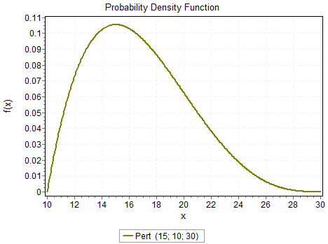
Figure 23.1: Pert Distribution
As you can see, this distribution ensures that our randomness is bound to realistic values. In this case, there are no negative values322, the distribution is usually skewed to the right, and the mode is less than the mean. We highly recommend this means of obtaining estimates, especially in the early modeling stages. The Triangular distribution can also be used to model the case when given the minimum, maximum, and most likely points. However, it will be heavier in the tails, while the Pert will have more probability around the mode.
With the liberal use of these kinds of estimates, build your simulation model. Vary some of the input model parameters (i.e., the mode, minimum, or maximum) and see the impact they have on the simulation outputs. In particular, note how they impact the simulation outputs that are important to you. With a little experimentation of this type – called a “sensitivity analysis,” you begin to get a sense of which data are most critical. You can marshal a data collection effort proportional to the input model’s importance. There are a number of hard-to-answer questions regarding data collection. Often, you can’t collect as much data as you would like, so you will need to consider the limitations of your data collection budget. You will want to collect as much data as you can, bearing in mind that not all data is equally important in the model.
23.2 Input Modeling: Selecting a Distribution to Fit Your Data
Once you begin the data collection effort, you can begin to select distributions that fit your data. Why do we want to select a distribution to fit the data and not simply use the data directly in the simulation model? First, the data is only a sample from a population and not the total population, so we don’t know precisely whether the sample completely represents the population from which it is sampled. Secondly, real data tends to be incomplete in that it doesn’t completely match the process being modeled. Third, we believe that there are enough standard statistical distributions from which to choose that will do a good job of modeling the “true” input process. So, we will look for a distribution to fit the data.
Fortunately, once we have some data, the process of finding a distribution to fit the data is somewhat routine. Here are the steps we will follow:
Collect data and put it into a spreadsheet
Identify candidate distributions
For each candidate distribution
- Estimate parameters for the candidate distributions
- Compare candidate distribution to histogram
- Compare the candidate distribution function to the data-based distribution function
Select the best representation of the input (the input model)
Candidate Distributions
Before going into much detail, it is useful to do a SIMIO “Help” on “distributions.” You will see descriptions of all the distributions that SIMIO supports. Presently, they include the standard “continuous” distributions of Beta, Erlang, Exponential, Gamma, JohnsonSB, JohnsonSU, LogLogistic, LogNormal, Normal, PearsonVI, Pert, Triangular, Uniform, and Weibull as well as the standard discrete distributions of Binomial, Geometric, NegativeBinomial, and Poisson. Also, there are empirical distributions called continuous and discrete, which represent data-based continuous and discrete distributions. You should spend some time looking through these distributions, so you have some sense of their “shape” and parameters. For instance, Figure 23.2 displays the Erlang from the SIMIO help.
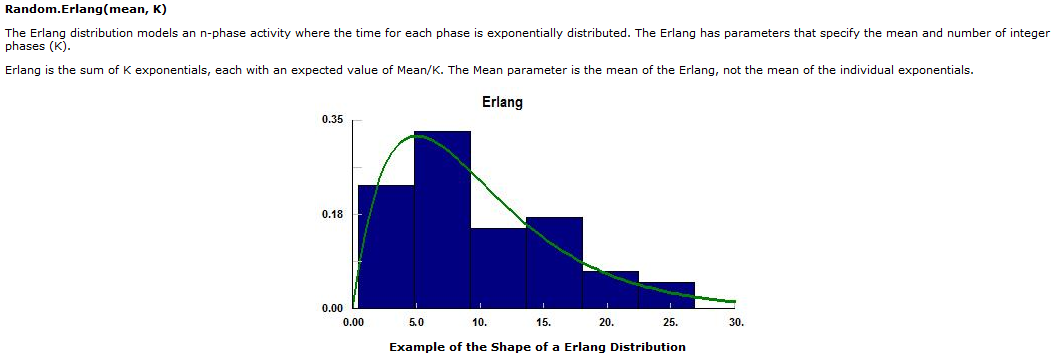
Figure 23.2: Erlang Distribution
The display shows that Erlang is a non-negative distribution specified by a mean and a number of phases (each phase being Exponentially distributed with a mean of the distribution divided by the number of phases).
In the prior figure, a histogram is displayed. A histogram is simply a display of the frequency in which data values fall within a given range. Typically, the ranges or cells of a histogram have identical ranges (sometimes the end cells are longer), and the number of histogram cells ranges from 5 to 15. The histogram is an arbitrary display since the user determines the size and number of cells, but some “rules of thumb” exist. For example, by dividing the range of observations (i.s., maximum – minimum) by the number of cells, you can determine the range for each cell. Although you would like to keep the number of cells, \(C\), between 5 and 15, the following can be a good guide:
Scott’s Rule: \(C \approx \displaystyle{\frac{5}{3}}n^{1/3}\)
Sturges’ Rule: \(C \approx 1 + 3.3 \log_{10}(n)\)
Here, the number of observations in your data is \(n\). With the range for each cell, you simply display the portion of the observations that fall within each range. By examining the histogram, you may want to select certain distributions to fit. But before you fit a distribution to the data, you need the parameters for the distribution, and they will need to be estimated from the data.
Estimating Distribution Parameters
The estimation of distribution parameters employs one of two methods: moment match and maximum likelihood. Moment matching requires that you know, for a two-parameter distribution, the mean and variance of the distribution in terms of its parameters. If the Erlang mean is given by the symbol \(\theta\) and there are \(k\) phases to the Erlang, then the
Mean = \(\theta\)
Variance = \(\displaystyle\frac{\theta^2}{k}\)
Therefore if you compute the average and the sample variance from your data as \(\overline{x}\) and \(s^2\), approximate mean by the average and the variable by the sample variance. Solving, you can approximate the parameters of the Erlang by the following equations
\(\theta = \overline{x}\)
\(k = \left(\displaystyle\frac{\overline{x}}{s}\right)^2\)
The method of “matching” the sample statistics to the parameter values is the essence of moment matching.
Maximum likelihood requires more statistical development than we wish to devote here. However, the basic idea is to find the parameters of the distribution so they have the greatest “likelihood” of coming from that parameterized distribution. Most statistical books that deal with “estimation” contain a description of maximum likelihood. In actual practice, the process of finding the maximum likelihood can become a computational challenge if done by hand, so using some kind of software to perform the computations is highly desirable. We do need to note that most statisticians prefer the use of maximum likelihood-to-moment matching for parameter estimation. The reasons are somewhat technical, but the general maximum likelihood will have the best parameter estimates (they are optimal in the sense that they produce the best unbiased, minimum variance estimates).
Determining Goodness-of-Fit
Once a candidate distribution has been identified and its parameters determined, you can now compare the distribution you fit to the data. Here is an example of a histogram with a candidate distribution (Lognormal) being displayed in Figure 23.3. The distribution parameters have been computed from the data.
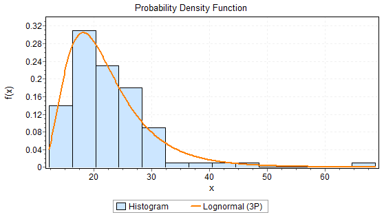
Figure 23.3: Probability Density Function
The basic question is how good is the “fit” of the Lognormal to this data? Our answer is based on two approaches: visual inspection and statistical tests.
Visual Inspection: Visual inspection is the most important strategy because it visualizes the fit. Looking at the prior histogram and the fitted distribution, it’s most important to see how the fitted distribution matches the observed histogram, particularly in the tails. The “tails” are most important because the variation in the distribution is largest in the tails, and the tails most generally affect the queuing, utilization, and flow time statistics.
Several other ways exist to “see” how well the fitted distribution matches the data. Most are based on the cumulative distribution function (CDF). For example, the comparison of the fitted CDF versus the data-based CDF is given in Figure 23.4.
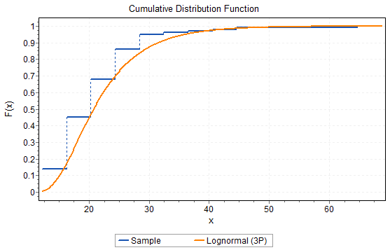
Figure 23.4: Cumulative Distribution Function
Again, we looked at how well the fitted distribution represents the data. When looking at the difference, it is useful to plot the difference in the two CDFs as in Figure 23.5
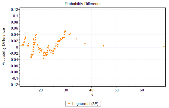
Figure 23.5: Difference between Empirical CDF and Fitted CDF
In this plot, we are looking to see if the difference is generally above or below 0, since that would indicate that the fit overestimates or underestimates the data.
Two of the more useful visual plots are based on the “distance” between the fitted CDF and the data-based CDF. If you measure the difference vertically, you obtain the PP plot, which emphasizes the difference in the center of the distribution. The PP plot is shown in Figure 23.6.
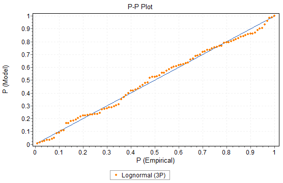
Figure 23.6: P-P Plot Example
If you measure it horizontally, you obtain the QQ plot, which emphasizes the difference in the tails of the distribution. The QQ plot is shown in Figure 23.7.
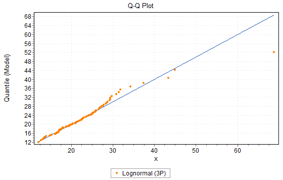
Figure 23.7: Q-Q Plot Example
In both the PP and QQ plots, we want to see the points “close” to the dividing line. Deviations from the line indicate a potential for overestimation or underestimation of the data. Finally, we tend to have more interest in the QQ plot than in the PP plot since it emphasizes the difference in the tails of the distribution, where we believe the fit is most important.
Statistical Tests: Statistical tests are based on classical statistical testing in which a null hypothesis is compared to an alternative. The null hypothesis is that the data comes from the fitted distribution. However, the “significance” of a statistical test is when the null hypothesis is rejected (Type 1 error). However, in goodness-of-fit, we want to accept the null hypothesis so the power of the test is relevant (Type 2 error); hence, we would like a larger p-value. Thus, statistical tests tend to reject only the poorest of fitted distributions. It is the reason we place so much emphasis on visual inspection.
There are three standard goodness-of-fit statistical tests: the Chi-Squared test, the Kolmogorov-Smirnov test, and the Anderson-Darling test. These tests are more thoroughly described in statistical texts. However, we can provide a general description of each.
The Chi-Squared test is based on comparing the observed number of observations in a histogram cell with the number expected if the fitted distribution was the input model. Although the test is often based on equal cell widths, it is generally better to use equal probability cells for the test.
The Kolmogorov-Smirnov (K-S) is a non-parametric test that looks at the largest (vertical) distance between the fitted CDF and the data-based CDF. The test is only approximate if parameters have to be estimated (which they usually are). A generalization of the K-S test is the Anderson Darling, which puts more weight in the tails of the difference (the K-S uses equal weights).
23.3 Distribution Selection Hierarchy
The following is a rule of thumb and represents the distribution selection hierarchy one should follow.
- Use recent data to fit the distribution using input modeling software
- Use raw data and load discrete points into a custom distribution (i.e., Empirical CDF)
- Use the distribution suggested by the nature of the process or underlying physics
- Assume a simple distribution and apply reasonable limits when lacking data (e.g., Pert or Triangular)
It is always better to fit distributions to data collected about the process. If no good fits can be achieved, the empirical distributions can be used to model the data. If some underlying distribution is suggested about the process owing to scientific processes, then one can utilize these. Assuming a simple distribution and applying reasonable limits can be used as a start if you have very little or no data. Often, we can obtain the minimum, maximum, and sometimes the most likely. In this case, we can use the Pert distribution.
23.4 Empirical Distributions in SIMIO
In contrast to the standard distributions, for which a functional form must be determined, parameters must be estimated, and empirical distributions are based totally on your data. You have two choices for empirical distributions: discrete and continuous. These distributions are represented in Figure 23.8, which describes the probability mass/density function as well as the cumulative distribution function.
The SIMIO statements for specifying discrete and continuous distributiosns as follows:
Random.Discrete(v1, c1, v2, c2, …,vn,cn)
Random.Continuous(v1, c1, v2, c2, …,vn,cn)

Figure 23.8: SIMIO Specification of Discrete and Continuous Distributions
Of the two distributions, the Discrete is the most often used. We might have a case where 30% have a value of 2.0, 50% have a value of 3.1, and 20% have a value of 6. A plot of this case is shown in Figure 23.9. Note that the sum of the probabilities is equal to 1.
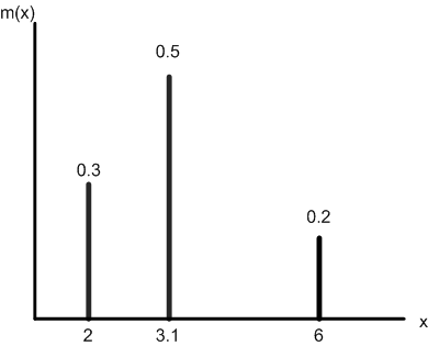
Figure 23.9: SIMIO specification: Random.Discrete(2, 0.3, 3.1, 0.8, 6, 1.0)
Some other examples of the use of the empirical discrete distribution in SIMIO are:
Random.Discrete(2, 0.3, Math.Epsilon +5.2, 0.8, 6, 1.0)
Random.Discrete(Random.Exponential(0.5),0.3,Run.TimeNow,0.8,6, 1.0)
Random.Discrete(“Red”,0.3,“Green”, 0.8, “Blue”, 1.0)
Of course, the value/expression can be negative, although it occurs infrequently. The cumulative probability parameters/expression must also be in the range 0 to 1, and the last cumulative probability parameter must be 1.
An example of continuous distribution might be where 30% of the time, the value falls (uniformly) between 1 and 2.5, 60% between 2.5 and 4, and 10% between 7 and 8. The plot for this case is shown in Figure 23.10.
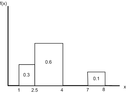
Figure 23.10: SIMIO Specification: Random.Continuous(1,0,2.5,0.3,4,0.9,7,0.9,8,1.0)
The values/expression should not decrease, although SIMIO does not check. Also, cumulative probability parameters/expression values must be in the range 0 to 1, and the last cumulative probability parameter must be 1.
23.5 Software for Input Modeling
The computational aspects of the distribution-finding process have been incorporated into the software. Several software “packages” exist now to help in fitting a distribution to data (SAS Jmp, ExpertFit, EasyFit, Minitab). The software will do the work of finding candidate distributions that represent the data.
Typical of input modeling software is EasyFit from http://www.mathwave.com. It comes with a free trial version, and a variety of licenses may be obtained. The software has a catalog of over 50 standard distributions. Data can be read from worksheets or entered and edited in the software’s worksheet. The fitting system considers all the distributions as possible candidates. However, The user may limit the fitting to (continuous) distributions with an upper or lower bound or both and whether these bounds are open or closed. Maximum likelihood estimates are used for distribution parameter estimation for each candidate distribution. The visual displays include the probability density (or mass) function, the cumulative distribution function, the PP and QQ plots, and the CDF difference plot. The histogram of the data can also specify the number of bins (cells). The statistical goodness-of-fit tests include the K-S, the Anderson-Darling, and the Chi-Squared with equal probability or equal width cells. The candidate distributions can be ranked by the statistics produced from the statistical tests.
Whenever you use input modeling software, you must be concerned with parameter correspondence between the software parameters and the SIMIO parameters. For example, the EasyFit parameters of Erlang\((m,\beta)\) correspond to Random.Erlang\((m*\beta,m)\) in SIMIO. Table 23.1 shows how to convert EasyFit parameters to SIMIO parameters.
| Distribution | Easy Fit | SIMIO |
|---|---|---|
| Bernoulli | Bernoulli(p) | Random.Bernoulli(p) |
| Beta | Beta(\(\alpha\),\(\beta\)) | Random.Beta(\(\alpha\),\(\beta\)) |
| Binomial | Binomial(nt,p) | Random.Binomial(p,n) |
| Erlang* | Erlang(m,\(\beta\)) | Random.Erlang(m*\(\beta\),m) |
| Exponential* | Exponential(\(\lambda\)) | Random.Exponential(\(\lambda\)) |
| Gamma* | Gamma(\(\alpha\),\(\beta\)) | Random.Gamma(\(\alpha\),\(\beta\)) |
| Geometric | Geometric(p) | Random.Geometric(p) |
| Johnson SB** | JohnsonSB(\(\gamma\),\(\delta\),\(\lambda\),\(\xi\)) | Random.JohnsonSB(\(\gamma\),\(\delta\),\(\xi\),\(\xi\)+\(\lambda\)) |
| Johnson UB(SU)** | JohnsonSU(\(\gamma\),\(\delta\),\(\lambda\),\(\xi\)) | Random.JohnsonUB(\(\gamma\),\(\delta\),\(\xi\),\(\lambda\)) |
| Log-Logistic* | Log-Logistic(\(\alpha\),\(\beta\)) | Random.LogLogistic(\(\alpha\),\(\beta\)) |
| Lognormal* | Lognormal(\(\sigma\),\(\mu\)) | Random.Lognormal(\(\mu\),\(\sigma\)) |
| NegativeBinomial | Neg.Binomial(n,p) | Random.NegativeBinomial(p,n) |
| Normal | Normal(stDev,mean) | Random.Normal(Mean,stDev) |
| PearsonVI* | Pearson6(\(\alpha 1\),\(\alpha 2\),\(\beta\)) | Random.PearsonVI(\(\alpha 1\),\(\alpha 2\),\(\beta\)) |
| Pert | Pert(m,a,b) | Random.Pert(a,m,b) |
| Poisson | Poisson(\(\lambda\)) | Random.Poisson(\(\lambda\)) |
| Triangular | Triangular(m,a,b) | Random.Triangular(a,m,b) |
| Uniform | Uniform(a,b) | Random.Uniform(a,b) |
| Weibull* | Weibull(\(\alpha\),\(\beta\)) | Random.Weibull(\(\alpha\),\(\beta\)) |
* Distributions that have a “Location” parameter but were not included in the syntax. For an example of how to use a location parameter in a SIMIO random variable distribution, see below.
** Distributions whose “Location” Parameters were indicated in the syntax to show how to derive some of the parameters in SIMIO of the same distribution.
For many distributions, EasyFit generates “location” parameters along with the distribution parameters. This location parameter permits a distribution to be located at some arbitrary point. If EasyFit provides a location, say \(\delta\), for the Erlang, then you will form the SIMIO expression:
\(\delta + Random.Erlang (m*\beta,m)\)
The location parameter is used to shift a distribution so it will not be based at zero.
23.6 The Lognormal Distribution
The Lognormal Distribution may require some explanation in case you want to use it. The Lognormal is defined as the distribution you get by taking the logarithm of a normally distributed random variable. That normal distribution defined with a mean \(\mu\) and a standard deviation \(\sigma\) is, in fact, the parameters of the SIMIO and the EasyFit Lognormal distribution. However, they are not the mean and standard deviation of the Lognormal distribution, which is given by:
LogMean \(= e^{\mu+\sigma^2/2}\)
LogStd \(= \sqrt{e^{2\mu+\sigma^2}\left(e^{\sigma^2}-1\right)}\)
If you have data from which you compute x and s, then you can compute SIMIO parameters (the Normal distribution parameters) from:
\(\mu \approx \ln \left(\overline{x}^2{\Large/}\sqrt{\overline{x}^2+s^2_x}\right)\)
\(\sigma \approx \sqrt{\ln\left( 1+s^2_x {\Large/}\overline{x}^2\right)}\)
23.7 Modeling the Sum of \(N\) Independent Random Variables
We are often faced with determining the processing time for a batch of parts to be processed individually. The processing time is, therefore, a sum of \(N\) independent random variables. For example, if there were 25 parts in a batch and each one took a \(Triangular(a, m, b)\) minutes to be processed, then the total time to process the batch is given by the summation of 25 independent triangular distributions as seen in the following equation.
\(Processing\ Time = \displaystyle\sum_{i = 1}^{25}{Triangular(a,m,b)}\)
Often, people will mistakenly model the processing time of summation of \(N\) independent random variables as \(N\) times the random variable of interest, which is incorrect as it does not correctly create the appropriate distribution, but it is easy to specify.
\(25*Triangular(a,m,b) \neq \displaystyle\sum_{i = 1}^{25}{Triangular(a,m,b)}\)
To illustrate the point, let’s take the Triangular distribution given a minimum value of \(a\), mode of \(m\), and a maximum value of \(b\). The mean and variance of this distribution are given by the following:
Mean \(= \displaystyle\frac{a + m + b}{3}\)
Variance \(= \displaystyle\frac{a^{2} + m^{2} + b^{2} - am - ab - bm}{18}\)
Because it is much easier to perform multiplication rather than summation, people will utilize the multiplication form given by the following equation.
\(N*Triangular(a,m,b) = Triangular(Na,Nm,Nb) \neq \displaystyle\sum_{i = 1}^{N}{Triangular(a,m,b)}\)
As one can see in Table 23.2 below, the means of the two different versions are the same. However, the variances are not. In other words, the modeling distribution is not what is desired. Figure 23.11 shows the PDF of each distribution; one can see that the true underlying distribution (i.e., summation distribution) is quite different. The reason is the variances of the summation of N independent variables add together rather than the standard deviations.
| Method | Equation |
|---|---|
| Summation Mean | \(\sum_{i = 1}^{N}{\left( \frac{a + m + b}{3} \right) = N\left( \frac{a + m + b}{3} \right)}\) |
| Summation Variance | \(\sum_{i = 1}^{N}{\left( \frac{a^{2} + m^{2} + b^{2} - am - ab - bm}{18} \right) = N}\left( \frac{a^{2} + m^{2} + b^{2} - am - ab - bm}{18} \right)\) |
| Multiplication Mean | \(\ \left( \frac{(Na) + (Nm) + (Nb)}{3} \right) = N\ \left( \frac{a + m + b}{3} \right)\) |
| Multiplication Variance | \(\left( \frac{{(Na)}^{2} + (N{m)}^{2} + (N{b)}^{2} - (Na)(Nm) - (Na)(Nb) - (Nb)(Nm)}{18} \right)\) |
| \(= N^{2}\left( \frac{a^{2} + m^{2} + b^{2} - am - ab - bm}{18} \right)\) |
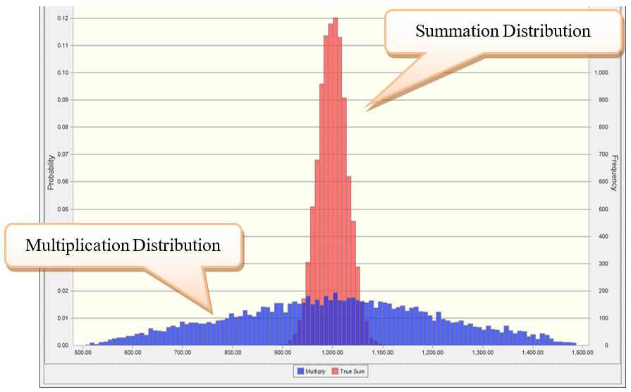
Figure 23.11: Comparing True Summation Distribution with the Multiplication Distribution
Correct Handling of Summation of \(N\) Independent Variables
The most appropriate method is to sample \(N\) random variables and then sum these values to reach the correct sample is to use the function
Math.SumOfSamples(randomExpression, numberofSamples)
You specify the random distribution (i.e., random Expression) and the number of samples needed. For example,
Math.SumOfSamples(Random.Triangular(10,15,20), 25)
Approximation for the Summation of \(N\) Independent Variables
As \(N\) gets large, the distribution that results from the summation of \(N\) independent distributions becomes Normal owing to the Central Limit Theorem. Therefore, given a large enough \(N\), the summation distribution can be approximated using a Normal distribution with the follownig mean and standard deviation (STD)
\(Normal\ Mean = N*Single\ Distribution\ Mean\)
\(Normal\ STD = \sqrt{N*Single\ Distribution\ Variance}=\sqrt{N}*Single\ Distribution\ STD\)
Figure 23.12 shows the exact summation distribution, the normal approximation, and the incorrect multiplication distribution. As you can see, the approximation is very good, given \(N\) was 25.
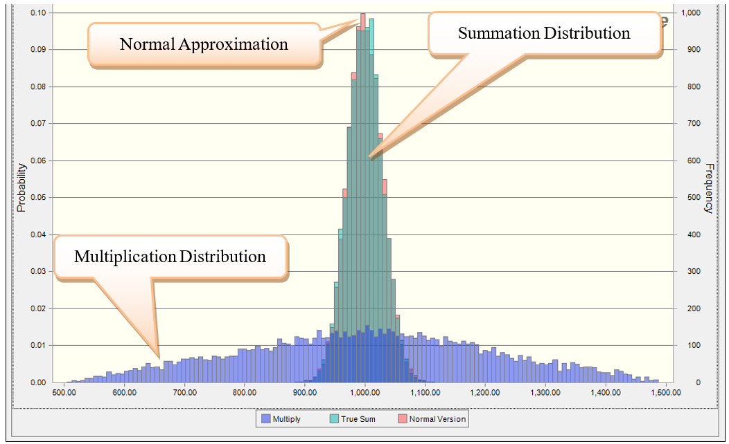
Figure 23.12: Simplified Normal Approximation versus the True Summation Distribution
The disadvantage of using the normal approximation is that the sampled values can become negative and the value \(N\) needs to be sufficiently large. Depending on the distribution, \(N< 10\) will not yield a very good normal approximation, and typically, \(N\) larger than 20 is sufficient.
If a sample from a distribution for a time, like a processing time, produces a negative value, SIMIO will display an error. Distributions that can have negative values, like the Normal must be used with care. You can avoid negative values using and expression like Math.Max(0.0, Random.Normal(10.0,4.0)):.↩︎