Simulation Modeling with Simio - 6th Edition
Chapter
4
More Detailed Modeling: Airport Revisited
There usually is more than one type of check-in in an airport and more than one type of passenger (i.e., a curbside check-in or a no-checked-bags check-in traveler). Our goal is to embellish the airport model from the last chapter to handle routing to different check-in stations, varying arrival rates of passengers, and varying types of passengers with rate tables and data tables. We will also introduce a means of giving entities characteristics, called state variables, which can be used to provide various distinctions.
4.1 Choice of Paths
As in the previous chapter, our primary concern is the amount of time it takes the passengers to reach the security checking station and the number of needed check-in stations.
4.1.1 Delete the Experiment object in the prior chapter model by right-clicking on the Experiment in the [Navigation] Panel.24 We will embellish the previous airport model to allow passengers arriving to choose three different routes to reach the security check. Passengers who need to check bags and get tickets can either check in at the curbside station (10%) or check in at the central station inside the airport (70%), while some passengers can proceed directly to the security checkpoint (20%). Refer to Figure Figure 4.1, which depicts the modified airline check-in process to be modeled.
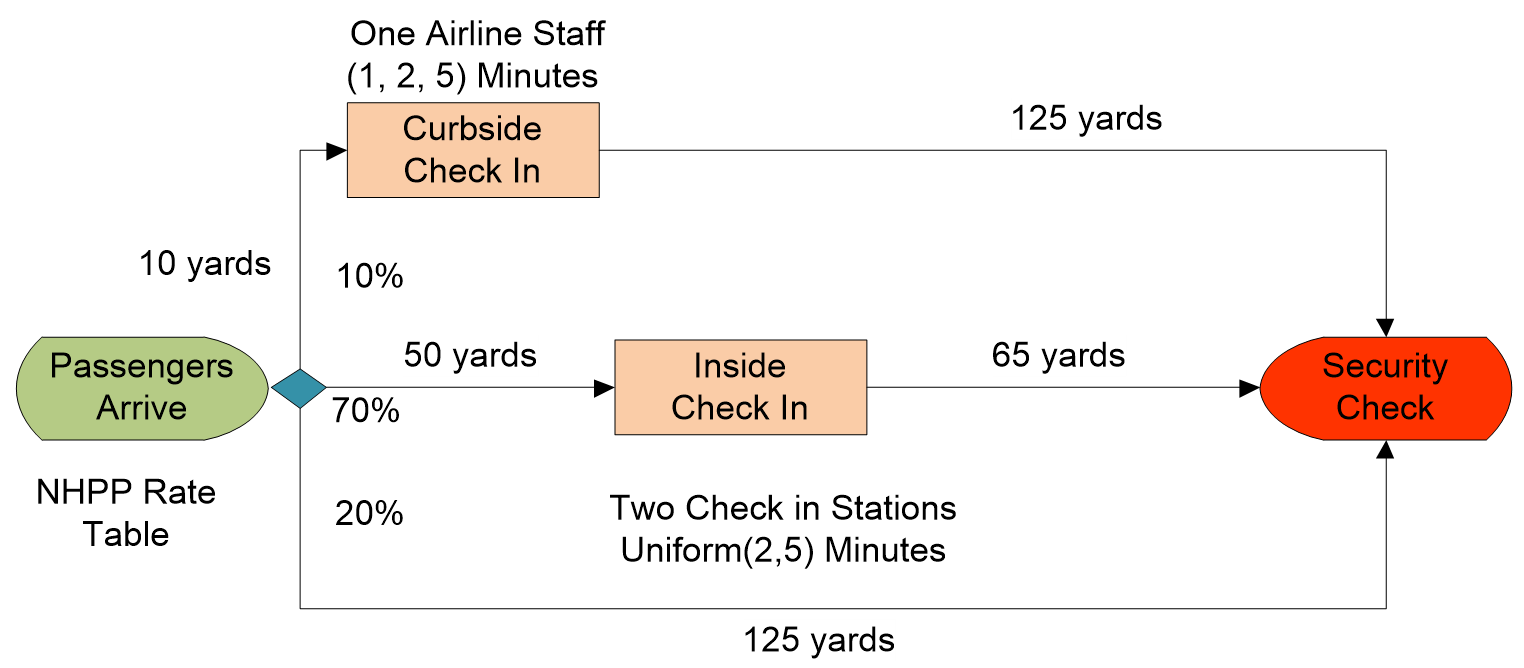
Figure 4.1: Modified Airline Check-in Process
Route 1: Passengers who use the curbside check-in need to walk 10 yards to reach the station, where a single airline staff member takes between one and five minutes, with a most likely time of two minutes, to check-in a passenger. Once they have checked in, they walk 125 yards to the security check line.
Route 2: Passengers who have checked in online do not need to check any luggage; they only need to walk 125 yards to the security check line once they arrive at the airport.
Route 3: Passengers who plan to use the inside check-in first must walk 50 yards to reach the station where there are currently two airline personnel (instead of four previously) checking passengers into the airport. It takes between three and ten minutes uniformly to process each passenger. Once they have checked in, they walk 65 yards to the security check line.
4.1.2 Modify the model from the last chapter to include the new curbside check-in (Server) and the direct path (i.e., Route 2) from the arrivals to the security gate, as seen in Figure 4.2. Specify the properties according to the description in Figure 4.1.
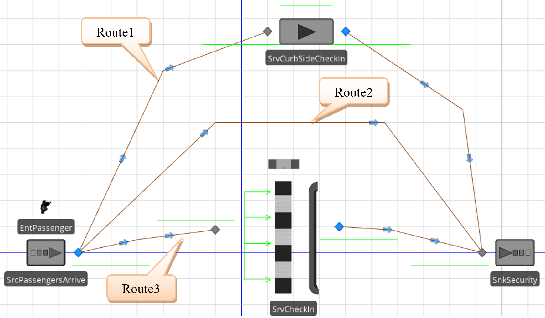
Figure 4.2: Creating Different Routing Paths
4.1.3 It has been observed that passengers follow the probabilities in Table 4.1 in determining which route they will take to reach security.
| Check-in Type | Percentage |
|---|---|
| Curbside Check-in | 10% |
| Inside Check-in | 70% |
| No Check-in (Carry on) | 20% |
4.1.4 To model the decision of a passenger in choosing their check-in route, the Selection Weight property of Path objects will be utilized. The probability of selecting a particular path is that the path’s individual selection weight is divided by the sum of all path selection weights from that node object. Place the proper weights on each check-in route (see Figure 4.3).
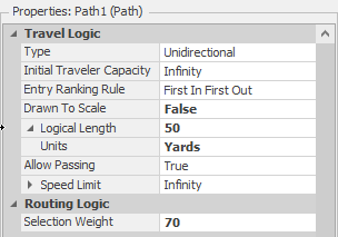
Figure 4.3: Weighting Paths
4.1.5 Remember to select the Outbound Link Rule to be “By Link Weight” on the TransferNode Output@SrcPassengersArrive (see Figure 4.4).25
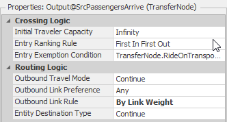
Figure 4.4: Outbound Link Rule
4.1.6 Run the model for one 24-hour replication (i.e., no “Experiment” needed). You might want to improve on our animation.
4.1.6.1 What is the average number of passengers waiting at Curbside and the Inside Check-in?
_______________________________________________
4.2 Changing Arrival Rate
Passengers do not arrive at a constant rate (i.e., homogeneous process) throughout the entire day in an actual airport (even though they may arrive randomly), so we should expand our model to handle such phenomena. Our approach will be to allow the arrival rates to change throughout the day. To model this changing rate, we will use a data object in SIMIO called a Rate Table and reference the Rate Table we create in the arrival logic of our Source object. It is essential to understand that the interarrival times for this rate will be assumed to be Exponentially distributed, but the mean of this distribution changes with time. If an interarrival process has an exponential distribution, then it is statistically known that the number of arrivals per unit of time is Poisson distributed. Since the parameter (i.e., the mean) changes with time, it is formally referred to as a “non-homogeneous Poisson” arrival process, also called a NHPP (Non-Homogeneous Poisson Process). Therefore, when you use a SIMIO Rate Table, you assume the arrival process is an NHPP. Table 4.2 shows the hourly rate over the 24-hour day, where more passengers arrive on average during the morning and dinner hours. The zero rates imply no arrivals during that time period.
| Begin Time | End Time | Hourly Rate |
|---|---|---|
| Midnight | 1:00 AM | 0 |
| 1:00 AM | 2:00 AM | 0 |
| 2:00 AM | 3:00 AM | 0 |
| 3:00 AM | 4:00 AM | 0 |
| 4:00 AM | 5:00 AM | 0 |
| 5:00 AM | 6:00 AM | 30 |
| 6:00 AM | 7:00 AM | 90 |
| 7:00 AM | 8:00 AM | 100 |
| 8:00 AM | 9:00 AM | 75 |
| 9:00 AM | 10:00 AM | 60 |
| 10:00 AM | 11:00 AM | 60 |
| 11:00 AM | Noon | 30 |
| Noon | 1:00 PM | 30 |
| 1:00 PM | 2:00 PM | 30 |
| 2:00 PM | 3:00 PM | 60 |
| 3:00 PM | 4:00 PM | 60 |
| 4:00 PM | 5:00 PM | 75 |
| 5:00 PM | 6:00 PM | 100 |
| 6:00 PM | 7:00 PM | 90 |
| 7:00 PM | 8:00 PM | 30 |
| 8:00 PM | 9:00 PM | 0 |
| 9:00 PM | 10:00 PM | 0 |
| 10:00 PM | 11:00 PM | 0 |
| 11:00 PM | Midnight | 0 |
4.2.1 Arrivals are only present from 5 am to 8 pm for a total of 15 hours each day. A simulation run length of 24 hours would cause the time-based statistics like number in station, number in queue, and scheduled utilization to be computed when there were no arrivals, causing lower than expected values for these statistics. Therefore, we will set the Starting Time within the “Run Setup” tab to 5:00 am and the Ending Type to Specific Ending Time at 8:00 pm, as shown in Figure 4.5
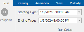
Figure 4.5: Replication Start and Stop Time
4.2.2 Select the “Data” tab to create a Rate Table and then click Create →Rate Table. Name the table PassengerArrivalRate. Set the Interval Size to one hour and the Number of Intervals to 15, corresponding to the run length as seen in Figure 4.6. While you can modify the size (e.g., half-hour increments) and number of time intervals during which the arrival rate is constant, you cannot change the rate, which is fixed at arrivals per hour.
4.2.3 Enter values in the rate table, as shown in Figure 4.6.
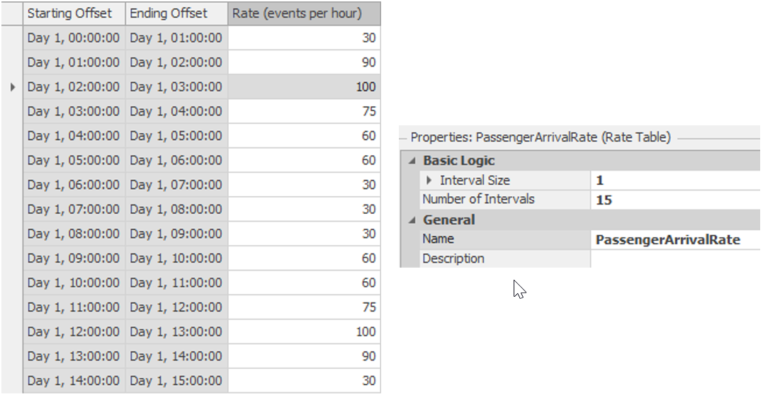
Figure 4.6: The Rate Table (15 intervals)
4.2.4 Modify the SrcPassengersArrive source accordingly (see Figure 4.7 for details). SIMIO refers to the NHPP as a “Time-VaryingArrival Rate” Arrival Mode.
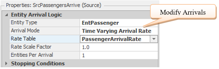
Figure 4.7: Specifying a Time-Varying Arrival Rate
4.2.5 Run the model and observe the results.
4.2.5.1 What are the average wait times at each check-in location (Curbside and Inside)?\newline
_______________________________________________
4.2.5.2 What is the average check-in time for a passenger (Curbside and Inside)?
_______________________________________________
If the simulation length (i.e., replication/run length) exceeds the size of the rate table, then the rate table repeats until the simulation replication is terminated. So, if the run length should be longer and there should be no arrivals during that time, then the rate table should contain zeroes accordingly.
4.3 State Variables, Properties, and Data Tables
Properties and state variables can be characteristics of the “Model” or the “Model Entities.” A “property” of an object is part of its definition and is assigned when an object is created, but it can’t be changed during the simulation. Properties can be expressions, so their evaluation and creation time can yield different values. In contrast, a “state variable” is a characteristic of an object that can be changed dynamically during the simulation. Generally, when properties and state variables are associated with the model, they are global because their values are visible throughout the model. When properties and state variables are associated with entities, you need to access the model entity to access the particular entity’s state variable value.
In an actual airport, more than one type of passenger arrives. Some are continental travelers, while others are inter-continental travelers. Still, some passengers have handicaps and require special attention or are with families. The different types of passengers result in additional processing times. To model these three cases, we will use a combination of state variables and properties to store the information and reference the information when needed.
There is a 33% chance for each type of passenger to arrive at our airport. The processing times at the curbside and inside check-ins vary depending on the passenger type. Specifically, see Table 4.3 for the processing times.
| Passenger Type | Curbside Check-In Time (minutes) | Inside Check-In Time (minutes) |
|---|---|---|
| 1 | Triangular(1, 2, 5) | Uniform(2, 5) |
| 2 | Triangular(2, 3, 6) | Uniform(3, 5) |
| 3 | Triangular(3, 4, 7) | Uniform(4, 6) |
The ModelEntity will need to reference these data as specifications at the various check-in counters.
4.3.1 Since the passenger type is not a general characteristic of SIMIO model entities, we need to find a SIMIO characteristic we can use to represent the type or define such characteristic ourselves. User-defined characteristics whose values can be re-assigned are the “State Variables.” A state variable can be a characteristic of the “Model” (namely global) or a characteristic of the “ModelEntity.” Here, we are interested in the characteristics of a ModelEntity.
4.3.2 To create a ModelEntity State Variable, select the “ModelEntity” object in the Navigation panel, as seen in Figure 4.8. Click the “States” panel icon in the ”Definitions” tab. It is convenient to number our passenger type, so select a Discrete “Integer” state from the ribbon. Let’s name it EStaPassengerType26. Next, we need to assign each ModelEntity a value for passenger type.
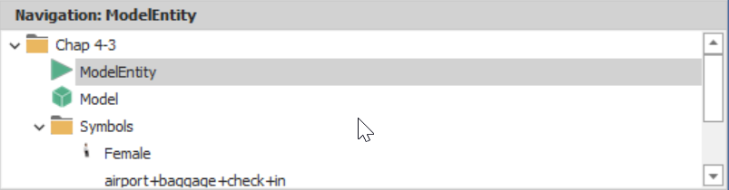
Figure 4.8: Selecting ModelEntity Object in the Navigation Panel
4.3.3 We need to assign a value to EStaPassengerType for each entity. To obtain a random assignment of passenger type to entities (i.e., 33% chance for each type), we must use the Discrete Distribution (entered in cumulative distribution form).
Random.Discrete(1, 0.33, 2, 0.66, 3, 1.00)
4.3.4 One convenient place is to make this assignment at the SrcPassengersArrive source object in the “State Assignments” property. Click on the plus box to reveal “Before Exiting.” Then click the ellipses box at the end of that specification to bring up the “[Repeating Property Editor,” which allows state value assignments in this case.
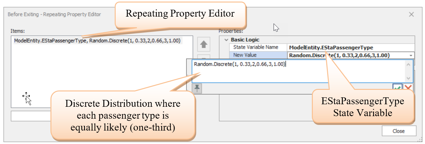
Figure 4.9: Assigning Passenger Type
Each passenger has a (randomly assigned) state variable that describes its passenger type.
4.3.5 To verify that the model behaves the way one intended, we often add labels to display information while the simulation is running. Let’s add a dynamic label to the entity to display the passenger type, as seen in Figure 4.10.
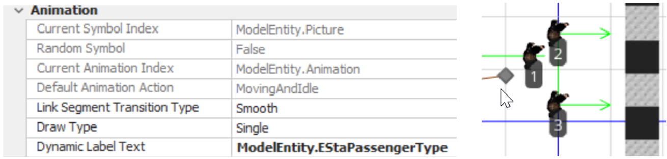
Figure 4.10: Creating a Dynamic Label to Display the Passenger Type
4.3.6 We need to store the information for the check-in times. The expression of these times (e.g., Random.Unform(2,5)) does not change throughout the simulation. These check-in times need to be accessed by all entities. The check-in times are not specific to each entity but are characteristics of the model. So, “properties” are an appropriate way to store these data for the model.
4.3.7 A way to organize model properties is through the use of a Data Table. The data table is functionally identical to the table we created for . To create a Data Table, click “Tables” in the ”Data” tab, then “Add Data Table.” Call it TablePassenger. Characteristics, called “properties,” can be added to the data tables – these properties are the columns in the table. In our Data Table, the processing times for each of the three types of passengers for each check-in location will be specified. Select the properties from the “Standard Property” option in the Properties section. PassengerPriority will be an Integer property, whereas the check-in times will be Expression properties named CurbsideCheckInTime and InsideCheckInTime.27 Priorities 1, 2, and 3 represent Continental, Inter-Continental, and special needs passengers, respectively, as in Figure 4.11.28
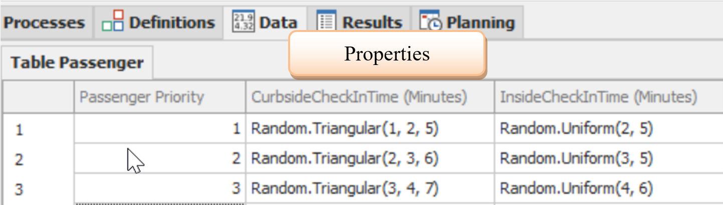
Figure 4.11: The Data Table
4.3.8 Since the check-in times are in minutes, we want to specify the “Unit Type” for these properties, as seen in Figure 4.1229.
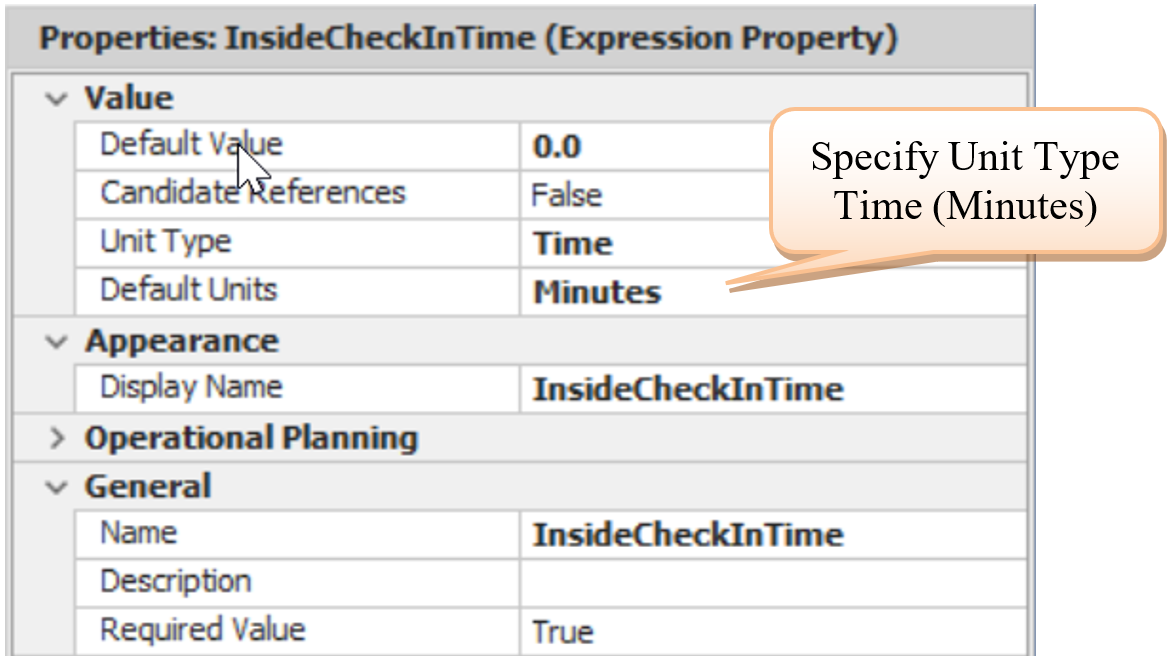
Figure 4.12: Inside Check-In Properties
4.3.9 Now, we must specify the processing times at the check-in stations to depend on the particular entity’s passenger type, as shown in Figure 4.13. The passenger type is used as the “row reference” in the table. Thus, the specifications needed for the new processing times use the EStaPassengerType state variable as:
- At SrvCurbSideCheckIn:30 TablePassenger[ModelEntity.EStaPassengerType].CurbSideCheckInTime
- At SrvCheckIn: TablePassenger[ModelEntity.EStaPassengerType].InsideCheckInTime
Notice that the content of the []31 is used to designate the specific row in the table, similar to arrays in programming languages. Unfortunately, the expression editor does not know about the Data Table properties since they are user-defined, so you must type the property into the expression. Also, be sure that the processing time units in the check-in stations are specified in minutes.
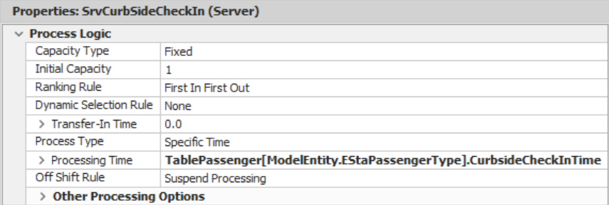
Figure 4.13: Utilizing the Table to Specify the Processing Times
4.3.10 Run the model. Remember, no arrival occurs before 5 am, and the simulation is started at 5 am, so no animation appears before then.
4.3.10.1 What are the average wait times at each check-in location (Curbside and Inside)?
_______________________________________________
4.3.10.2 What is the average check-in time for a passenger (Curbside and Inside)?
_______________________________________________
Properties and State Variables: Before leaving this section, let’s reflect on the characteristics of “properties” and “state variables” because they will be used frequently. Properties and state variables can be characteristics of the Model or the ModelEntities. A “property” of an object is a part of the object’s definition and is assigned at the time an object is created, but it can’t be changed during the simulation. Properties can be expressions, so their evaluation can yield different values. In contrast, a “state variable” is a characteristic of an object that can be changed during the simulation. Generally, when properties and state variables are associated with the model, they are global in the sense their values can be obtained almost anytime. When properties and state variables are associated with entities, you need access to that model entity to access the value.
SIMIO extensively uses properties and state variables, which you can see by looking at their “definitions” and expanding the (Inherited) Properties/States. Some properties and states are related. For example, the “InitialPriority” property of a ModelEntity becomes the initial value of the “Priority” state variable. Properties can be used to give other states their initial values.
4.4 More on Branching
At times, the waiting lines at the inside Check-in station seem overcrowded. We decided to add a second Inside Check-in station that passengers can use during rush hours. Thus, passengers will be routed to whichever check-in station has the smallest number in the waiting queue. The distance from this second Check-in station to the Security Check is 75 yards, as seen in Figure 4.14.
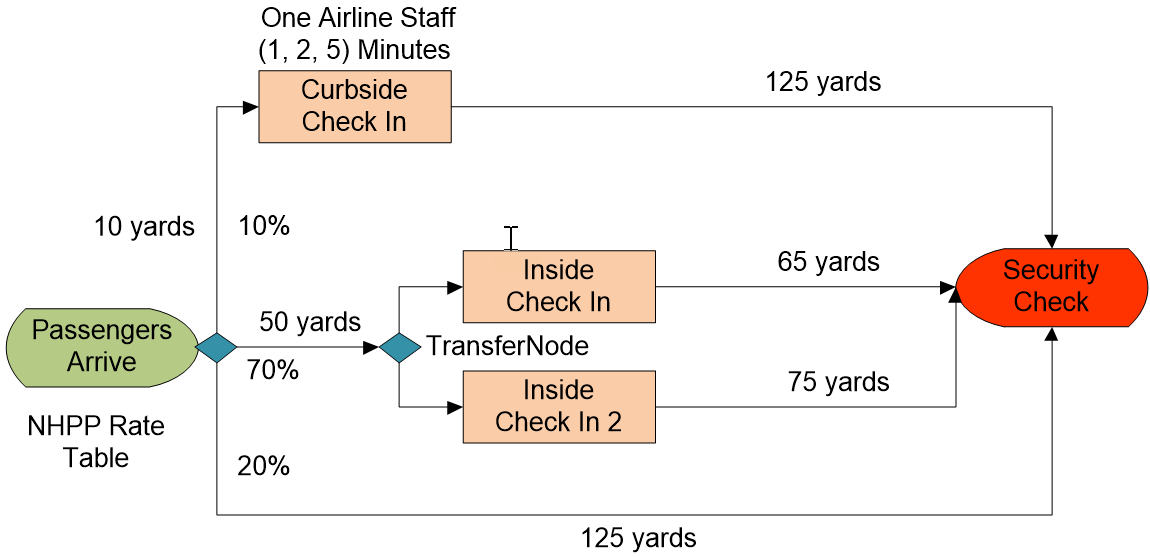
Figure 4.14: Airline Check-in Process with Two Inside Check-In Stations
4.4.1 Add the second check-in station by copying and pasting the current InsideCheckIn. Call it SrvCheckIn2. Assume it has a capacity of one, and its processing times are the same as those for the regular check-in station. Add the path of 75 yards from this second station to SnkSecurity.
4.4.2 We need to model the choice made by the “inside” check-in passengers to go to the check-in station with the smallest number in the queue. There are several ways to model this situation. Perhaps the most obvious or most straightforward way is to add a TransferNode that branches passengers to the shortest queue.
Delete the original path to the SrvCheckIn object from the SrcPassengersArrive.
Insert a TransferNode near both the check-in servers and a path from the SrcPassengersArrive to the TransferNode, ensuring the distance from the SrcPassengersArrive to this TransferNode is 50 yards. Also, remember that the selection weight is 70 for this path.
Next, connect the TransferNode to the two check-in servers’ input nodes using Connectors, which will take up zero time and space.
The TransferNode should specify the Outbound Link Rule as “By Link Weight.” If you leave it as the “Shortest Path,” it will use the selection weights since we have not specified a specific node for the entity to transport to.
Set the Selection Weight properties of the two paths from the TransferNode (the “value” of a “true” expression is one and zero if it is “false”)
To SrvCheckIn:
SrvCheckIn.InputBuffer.Contents.NumberWaiting <=
SrvCheckIn2.InputBuffer.Contents.NumberWaitingTo SrvCheckIn2:
SrvCheckIn2.InputBuffer.Contents.NumberWaiting <
SrvCheckIn.InputBuffer.Contents.NumberWaiting
4.5 Work Schedules
Suppose you decide only to staff the second inside check-in station from 10 am to 6 pm. This kind of concern requires a work schedule that alters the capacity of a server over time. Work schedules will be built from the “Schedules” component under the “Data” tab.
4.5.1 Click on the “Work Schedule” button under the “Schedules” icon in the “Data” tab to add a new work schedule. The StandardWeek schedule has already been defined by default, as seen in Figure 4.15. Rename this schedule SecondCheckInStation. Change the Days to “1” – this schedule will repeat daily.32 For each day of the work schedule, you need to specify the work pattern for that day. Therefore, you can have different patterns for different days (i.e., weekends, etc.). The StandardDay pattern was specified for Day 1. The Start Date property can be left as the default since we have a daily pattern.
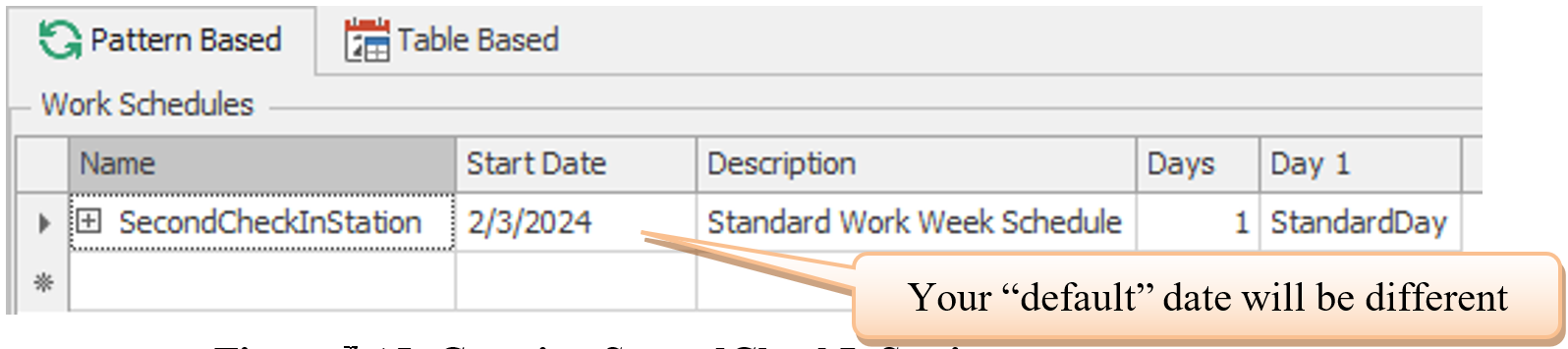
Figure 4.15: Creating aSecond CheckInStation WorkSchedule
4.5.2 In the “Day Patterns” section, you can add Day Patterns by clicking the Day Pattern button in the “Create” section. SIMIO defines the *StandardDay** pattern as 8 am to 5 pm with an hour lunch at 12 pm. We only need one work period in the pattern since we start the day at 10 am and end at 6 pm. Select and delete the second work period (1 pm to 5 pm). Then specify the Start Time to be 10 am, the Duration to be eight hours, or the “End Time” to be 6 pm, as seen in Figure 4.16. Specify a “1” for the Value, which will specify the capacity of the second inside check-in to be one. If a work period has not been defined for a period in the day pattern, it is assumed to be off shift (i.e., zero capacity).
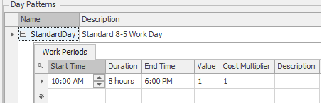
Figure 4.16: Setting a Day Pattern with Different Work Periods
4.5.3 Go to the “Facility” view and click on the SrvCheckin2 object. Change the Capacity Type to “WorkSchedule” and the Work Schedule property to *SecondCheckInStation** as in Figure 4.17.
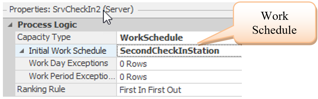
Figure 4.17: Specifying a Work Schedule
4.5.4 Now, we need to be sure that people who choose the inside check-in only go to the SrvCheckIn2 station if it is open (i.e., only between hours 10 and 18). This requires another TransferNode, as seen in Figure 4.18. Connect the original TransferNode to the new one via a Connector and connect the new TransferNode to the inputs of both check-in stations.
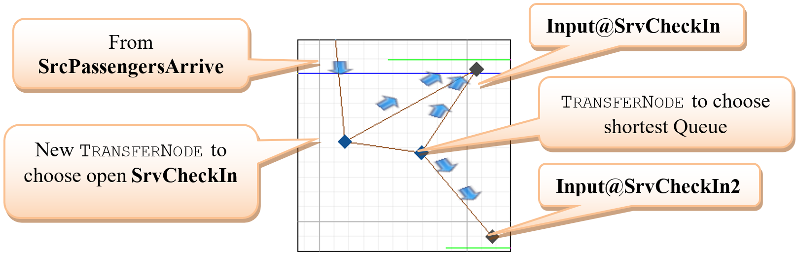
Figure 4.18: Adding Another TransferNode to Handle the Logic
- The new TransferNode should determine routing By Link Weight as well.
- Path to Input@SrvCheckIn has zero length33 and Selection
Weight property:
Run.TimeNow <=5 || Run.TimeNow>=1334 - Path to TransferNode to choose the shortest queue has zero length and Selection Weight property of Run.TimeNow > 5 && Run.TimeNow <1335
4.5.5 Note that the default time units are hours when there is no context. Now, run the model and obtain these basic statistics.
4.5.5.1 What is the average Check-In time for a Passenger?
_______________________________________________
4.5.5.2 What is the average wait time for Curbside Check-In?
_______________________________________________
4.5.5.3 What are the average wait times for two inside Check-In stations?
_______________________________________________
4.5.6 You may have noticed that in the simulation, there are entities in the queue of the SrvCheckIn2 that are in line when the station closes. These are marooned in this model. We will consider how to handle this kind of problem in a later chapter.
4.5.7 If we want to determine the best starting and ending times to open up the second check-in station, the link weights using the Run.TimeNow expression would have to be changed to match the new start and end times each time. A better approach would be to use the server’s capacity so that as it goes to zero, we need to close the path and open it when the capacity goes to one. Change the link weights according to and rerun the model, comparing the previous results.
- Path to Input@SrvCheckIn Selection Weight property: SrvCheckIn2.Capacity == 036
- Path to TransferNode to choose the shortest queue has zero length and Selection Weight property of SrvCheckIn2.Capacity > 0
4.6 Commentary
- With the very high utilization and long wait times, one would use the model to determine the appropriate capacity at each inside check-in station to make the waiting time reasonable.
- Specifying the time-varying arrival pattern in SIMIO requires fixed units for the arrival rate, namely arrivals per hour.
- Please pay special attention to the SIMIO specification of cumulative probability and its value for the Random.Discrete and Random.Continuous distributions.
- While work schedules in SIMIO offer considerable flexibility in specifying exceptions, etc., they are somewhat complicated to input. One has to be careful when specifying the correct times and duration. Also, be cautious when specifying the time to begin and end the simulation run.
- In SIMIO, when a server’s capacity goes to zero while there is an entity (or entities) being processed, SIMIO chooses, by default, to “Ignore” this so that the items “in process” will be processed while at the same time, the server capacity goes to zero. If another behavior is desired, then you will need to implement it using more advanced concepts, which will be described later.
- Note that if the length of the simulation replication exceeds the work schedule time, the work schedule is repeated until the replication ends.
The Navigation Panel in the upper right corner contains all of the models, objects, and experiments in the project. You can access the properties, rename the item, or delete the item from the project.↩︎
Although “Shortest Path” is the default Outbound Link Rule, the “By Link Weight” rule will still be used unless the entity destination has been assigned to a particular node using by “Sequence, Specific, or Select from List” on the Entity Destination Type. Therefore, we could have used the default rule.↩︎
We will use “E” to when denoting “Entity” and “Sta” to denote “State variable”.↩︎
Note that if you first specify the “General” name, it will become the default for the “DisplayName” property. Also, by using proper case, the table labels as seen in the Figure 4.10 will have spaces between the words.↩︎
Even though the check-in times are expression properties, the familiar drop down expression editor is not available in Data Tables. Therefore, the easiest way is to put in all three priorities and type in the first value of the first row. Then copy it to the other rows and just modifying the values of the parameters.↩︎
It may seem obvious the Unit Type for the time properties should be specified. However, one can leave the units as unspecified then the numbers will take on the units of the property when they are used (i.e., default value of hours).↩︎
To enter this specification to employ the expression editor during entry is to first put in the table name and property as TablePassenger.CurbSideCheckInTime and then insert [ModelEntity.EstaPassengerType]. In later chapters, we will not use this approach but directly assign a row in the table directly to the entity.↩︎
Note: table rows start at one (i.e., the first passenger type check in time is TablePassenger[1].InsideCheckInTime)↩︎
If there are seven days in the pattern, then the days of the week will appear. In our case there is only the Day 1 pattern. SIMIO will repeat the pattern based on the number of days in the Work Schedule. For each day in the work schedule you need to specify a pattern. Also, we have the ability to specify exceptions to the day pattern or work periods for particular dates.↩︎
May be easier to use a Connector instead of a Path – Connectors have zero length and take zero time to traverse.↩︎
Note, SIMIO utilizes || as the “Or” logical operator and && as the “And” logical operator. Also, this expression works only here since we are simulating just one day and 10 A.M. represents five hours into the simulation since we are starting at 5 A.M. If we were simulating more than one day, then we would need to specify Math.Remainder(Run.TimeNow, 24)*24 which converts the running time into a number between 0 and 24.↩︎
We could have modified the original link weights and avoided having to add the new paths and transfer node.
Specify the expression to be ((TimeNow <=5 || TimeNow >= 13) || SrvCheckIn.InputBuffer.Contents.NumberWaiting <= SrvCheckIn2.InputBuffer.Contents.NumberWaiting for the link weight for the path to SrvCheckIn and for the path link weight to SrvCheckin2 to (TimeNow >5 && TimeNow < 13) && SrvCheckIn2.InputBuffer.Contents.NumberWaiting < SrvCheckIn.InputBuffer.Contents.NumberWaiting.↩︎Note, SIMIO utilizes a double equal sign (i.e., “==” as the logical equal.↩︎